Digital Elevation Models: Creation and Applications

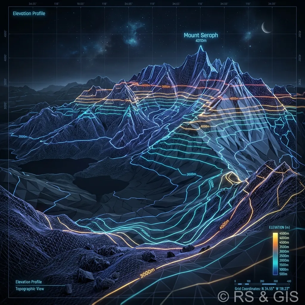
In the rapidly evolving fields of geospatial science, remote sensing, and civil engineering, Digital Elevation Models (DEMs) serve as the foundational bedrock for three-dimensional topographic analysis. A DEM is a quantitative, digital representation of the Earth's surface—or any other terrestrial planet—providing precise elevation values (Z) for a continuous grid of geospatial locations (X, Y). From mitigating catastrophic flood risks to designing billion-dollar infrastructure projects, the accuracy and fidelity of a DEM are paramount.

This comprehensive guide delves deep into the mathematical underpinnings, creation methodologies, interpolation algorithms, and far-reaching applications of Digital Elevation Models. Whether you are a GIS professional, a hydrologist, or a remote sensing specialist, mastering the intricacies of DEMs is essential for unlocking the full potential of spatial data.

1. Demystifying the Terminology: DEM vs. DTM vs. DSM

Before exploring the technical nuances of creation and application, it is critical to untangle the often-confused acronyms in elevation modeling: DEM, DTM, and DSM. While sometimes used interchangeably in casual conversation, they hold distinct semantic and mathematical definitions in Geographic Information Systems (GIS).

Model Type	Acronym	Definition & Characteristics	Primary Use Cases
Digital Elevation Model	DEM	A generic term for any digital representation of a topographic surface. Frequently used interchangeably with DTM in the US, representing the "bare earth" free of vegetation and structures.	General terrain analysis, global datasets (SRTM, ASTER).
Digital Surface Model	DSM	Captures the highest elevation points of the landscape. This includes natural and built features such as tree canopies, buildings, bridges, and powerlines.	Line-of-sight analysis, 3D city modeling, aviation planning, forest canopy estimation.
Digital Terrain Model	DTM	Specifically represents the bare ground surface, computationally stripped of all vertical extrusions (trees, buildings). Often augmented with breaklines and spot heights for higher fidelity.	Hydrological modeling, flood inundation mapping, cut-and-fill volume calculations.

Mathematically, one can often derive structural heights (like tree canopies or building heights) using a simple map algebra operation: Canopy Height Model (CHM) = DSM - DTM.

2. The Mathematical Anatomy of a DEM

At its core, a Digital Elevation Model is a matrix of numerical values. There are two primary spatial data structures used to encode this topographic information: Raster grids and Triangulated Irregular Networks (TINs).

2.1 Raster Grids

The vast majority of DEMs are formatted as raster grids. A raster divides the world into discrete, equally sized square cells (pixels). Each pixel is assigned a single numerical value representing the mean or central elevation of that area.

• Spatial Resolution: Defined by the ground footprint of a single pixel (e.g., 30-meter, 1-meter, or sub-centimeter). Higher resolution equates to smaller pixel sizes, capturing micro-topography but exponentially increasing file size and computational overhead.
• Bit Depth: Most modern DEMs utilize 32-bit floating-point data types to allow for highly precise decimal elevation values, minimizing vertical step-artifacts seen in older 8-bit or 16-bit integer models.

2.2 Triangulated Irregular Networks (TINs)

Unlike regular raster grids, TINs are vector-based topological data structures. They represent the terrain as a continuous surface of non-overlapping, contiguous triangles. The vertices of these triangles are the actual measured XYZ points.

• Delaunay Triangulation: TINs are generated using Delaunay triangulation algorithms, maximizing the minimum angle of all triangles to avoid long, skinny triangles that distort terrain representation.
• Variable Resolution: TINs are exceptionally efficient because they allow for variable point density. Flat plains can be modeled with a few large triangles, while complex cliffs and ridges can be densely packed with thousands of small triangles.

3. Technologies for DEM Creation and Data Acquisition

The creation of a high-fidelity DEM begins with robust data acquisition. The choice of sensor determines the spatial resolution, vertical accuracy, and appropriate application of the resulting model.

3.1 Light Detection and Ranging (LiDAR)

LiDAR has revolutionized DEM creation. Mounted on aircraft (ALS), drones (UAV), or terrestrial tripods (TLS), a LiDAR scanner emits hundreds of thousands of laser pulses per second. By measuring the time of flight (ToF) for the laser to bounce back to the sensor, the system calculates exact XYZ coordinates.

Crucially for DTM creation, LiDAR allows for multiple returns. A single laser pulse might hit the top of a tree canopy (first return, used for DSM), branches inside the canopy (intermediate returns), and finally the ground itself (last return). Complex filtering algorithms—such as Progressive Morphological Filters (PMF) or Cloth Simulation Filtering (CSF)—are then applied to strip away vegetation and generate a pristine bare-earth DTM.

3.2 Aerial and UAV Photogrammetry

Photogrammetry involves taking overlapping 2D photographs and using complex geometry to extract 3D measurements. Modern Structure-from-Motion (SfM) algorithms automatically identify millions of common tie-points across overlapping images.

By computing the internal and external orientation of the cameras at the time of each photograph, SfM software triangulates the intersection of these light rays to produce dense 3D point clouds. While highly cost-effective and capable of incredible resolution, photogrammetry primarily generates DSMs, as optical cameras cannot penetrate dense forest canopies like LiDAR lasers can.

3.3 Synthetic Aperture Radar (SAR) and Interferometry (InSAR)

For global and regional scale DEMs, radar is king. Radar sensors emit microwave energy which can penetrate cloud cover and operate day or night. Interferometric SAR (InSAR) uses two or more SAR images taken from slightly different sensor positions.

By analyzing the phase difference (interference pattern) between the returning radar waves, scientists can calculate the precise topography. This technique was the backbone of the Shuttle Radar Topography Mission (SRTM), which mapped the majority of the Earth's landmass in 11 days.

3.4 Traditional Ground Surveying

For projects requiring absolute, millimeter-level precision (such as foundation engineering or dam construction), traditional surveying techniques using Total Stations and Real-Time Kinematic (RTK) GPS receivers remain indispensable. While slow and labor-intensive, these methods provide the ground-truth data often used to calibrate and validate LiDAR and photogrammetric DEMs.

4. Processing and Spatial Interpolation Algorithms

Raw elevation data rarely comes in a perfect grid. Point clouds generated by LiDAR or SfM are scattered irregularly. To create a raster DEM, these points must undergo spatial interpolation—a mathematical process of estimating the elevation values of unknown locations based on known surrounding data points.

4.1 Inverse Distance Weighting (IDW)

IDW is a deterministic interpolation method based on Tobler’s First Law of Geography: "Everything is related to everything else, but near things are more related than distant things." In IDW, the value of an unknown grid cell is calculated as a weighted average of nearby points, with the weights being inversely proportional to the distance. It is computationally fast but can create "bullseye" artifacts around isolated data points.

4.2 Spline Interpolation

Spline fits a mathematically defined, flexible two-dimensional surface through the known input points. Imagine stretching a rubber sheet over a series of pegs of varying heights. Spline interpolation minimizes the overall surface curvature, resulting in a smooth, aesthetically pleasing DEM. It is excellent for gently rolling terrain but can create exaggerated, unrealistic "overshoots" in areas with extreme elevation changes, like cliffs.

4.3 Kriging

Kriging is a powerful geostatistical interpolation method. Unlike IDW, which only looks at distance, Kriging analyzes the spatial autocorrelation of the dataset. It fits mathematical models (spherical, exponential, Gaussian) to an empirical semivariogram, defining the variance between data points as a function of distance. Kriging not only produces a highly accurate DEM but also generates a predictive error surface, quantifying the uncertainty of the interpolated elevations.

4.4 Topo to Raster (ANUDEM)

Developed specifically for creating hydrologically correct DEMs, the Topo to Raster algorithm (based on the ANUDEM program) interpolates elevation while simultaneously enforcing drainage constraints. It explicitly removes artificial sinks and depressions, ensuring that simulated water can flow continuously across the landscape without getting trapped in mathematically generated pits.

5. Crucial Applications of Digital Elevation Models

The true value of a DEM lies in its derivatives. By processing a DEM through spatial algorithms, professionals unlock a vast array of analytical applications across diverse scientific and engineering disciplines.

5.1 Hydrology and Watershed Management

DEMs are the absolute backbone of computational hydrology. From a high-resolution DTM, GIS software can extract the structural framework of an entire river basin. Key hydrologic derivatives include:

• Flow Direction: Calculates the direction water will flow out of each pixel using the D8 (deterministic eight-node) algorithm, sending water to the steepest down-slope neighbor.
• Flow Accumulation: Counts the number of upstream pixels flowing into a given cell. High accumulation values mathematically define stream networks and river channels.
• Watershed Delineation: By defining a "pour point" (e.g., a dam location or river mouth), algorithms can trace back all contributing topography to map the precise boundaries of the watershed.
• Flood Inundation Modeling: Combining DEMs with hydrological flow models (like HEC-RAS) allows engineers to simulate rising water levels, mapping the exact extent and depth of 100-year and 500-year floodplains to mitigate disaster risks.

5.2 Geomorphology and Topographic Analysis

Geologists and soil scientists use DEMs to quantitatively analyze the shape and structure of the Earth’s surface.

• Slope: Calculates the maximum rate of change in elevation between a pixel and its neighbors, expressed in degrees or percent rise. Crucial for assessing landslide susceptibility and construction feasibility.
• Aspect: Identifies the compass direction that a topographic slope faces. Aspect analysis is vital for agriculture (determining microclimates for vineyards), solar panel placement, and modeling snowmelt rates in mountainous regions.
• Curvature: Measures the second derivative of the surface, calculating whether a slope is convex or concave. Profile curvature affects flow acceleration (erosion), while planform curvature affects flow convergence (water pooling).

5.3 Civil Engineering and Infrastructure Planning

No modern highway, railway, or pipeline is designed without a highly accurate DEM.

• Cut-and-Fill Volume Calculations: By comparing a pre-construction DEM with a proposed design DEM, engineers can exactly calculate the cubic volumes of earth that need to be excavated (cut) or added (fill). Balancing these volumes minimizes the expensive transport of dirt off-site.
• Line-of-Sight and Viewshed Analysis: Evaluates visibility from a specific point. This is heavily used in telecommunications for positioning 5G cell towers, in military operations for threat assessment, and in urban planning to protect scenic viewpoints.
• Route Optimization: Least-cost path algorithms traverse DEMs to find the most efficient route for roads or pipelines, minimizing steep grades and reducing construction costs.

5.4 Forestry and Precision Agriculture

The interplay between a DSM and a bare-earth DTM is transformative for vegetation management.

• Biomass Estimation: Subtracting a DTM from a LiDAR-derived DSM yields a Canopy Height Model (CHM). Foresters use CHMs to isolate individual trees, measure timber volumes, estimate carbon sequestration, and plan selective logging operations.
• Precision Farming: High-resolution UAV DEMs allow farmers to identify micro-depressions in their fields that are prone to waterlogging. This data drives the installation of sub-surface drainage tiles and informs variable-rate irrigation systems, maximizing crop yields while conserving water.

6. Global DEM Datasets: The Gold Standard

For large-scale, continental, or global analysis, researchers rely on a few foundational public datasets that have progressively mapped the Earth.

• SRTM (Shuttle Radar Topography Mission): Flown in 2000, SRTM provided a near-global DEM at 30-meter (1 arc-second) resolution. Despite its age, it remains a heavily cited baseline dataset.
• ASTER GDEM: Created from millions of optical stereo pairs captured by the Terra satellite, ASTER offers 30-meter resolution covering 99% of the globe.
• Copernicus DEM (GLO-30): A highly accurate, edited global DEM derived from the TanDEM-X radar mission, offering exceptional vertical accuracy free of charge.
• EarthDEM & ArcticDEM: Utilizing supercomputing clusters to process vast amounts of commercial optical satellite imagery, these projects are generating time-stamped, 2-meter resolution elevation models, enabling scientists to measure volumetric changes in glaciers and coastlines over time.

7. Future Horizons in Elevation Modeling

The creation and application of Digital Elevation Models are undergoing rapid technological shifts. The integration of Artificial Intelligence (AI) and Machine Learning (ML) is dramatically improving the filtering of point clouds. Deep learning neural networks are now capable of identifying and extracting buildings and trees from photogrammetric DSMs to generate "synthetic" DTMs in areas where LiDAR is too expensive.

Furthermore, the miniaturization of LiDAR sensors has led to the proliferation of drone-based mapping. What once required a million-dollar aircraft operation can now be accomplished by a surveying team with a $15,000 UAV, producing sub-centimeter accuracy DEMs on demand. Combined with cloud-based geoprocessing platforms like Google Earth Engine, analyzing petabytes of elevation data globally is now accessible to researchers anywhere in the world.

Conclusion

Digital Elevation Models are far more than mere 3D pictures; they are highly complex mathematical matrices that form the geometric foundation of geospatial analysis. From the physics of laser pulses bouncing off the forest floor to the complex differential equations defining a watershed, the creation of a DEM requires an interdisciplinary convergence of surveying, computer science, and geography. As remote sensing technologies continue to achieve unprecedented resolutions and global coverage, the applications for DEMs will only continue to expand, offering deeper insights into the dynamic surface of our planet.