Advanced Terrain Synthesis and Digital Elevation Models

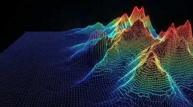
Terrain synthesis for Digital Elevation Models (DEMs) represents a critical intersection of computational geometry, applied mathematics, geomorphology, and computer graphics. The objective of terrain synthesis is to algorithmically generate or augment topographic surfaces that mimic the visual and statistical properties of real-world landscapes. These synthetic DEMs are pivotal across numerous domains, from hydrological simulations and ecological modeling to synthetic data generation for machine learning and expansive procedural environments in computer graphics.

A Digital Elevation Model is fundamentally a discrete representation of a continuous topographic surface. In its most common form, a DEM is structured as a regular two-dimensional grid (a raster) where each cell, or pixel, contains an elevation value representing the height of the terrain at that specific geographic coordinate. Synthesizing these models requires algorithms that can populate this grid with values exhibiting appropriate spatial autocorrelation, localized heterogeneity, and macro-scale geomorphological features such as mountain ridges and river valleys.

1. Procedural Noise and Fractional Brownian Motion (fBm)

The foundational bedrock of procedural terrain synthesis lies in gradient noise functions, most notably Perlin Noise and Simplex Noise. Unlike pure white noise, which lacks spatial correlation and appears chaotic, gradient noise produces pseudo-random gradients at integer lattice points and interpolates between them. This results in a continuous, differentiable surface that exhibits natural-looking undulations.

Mathematically, given a point \( P \) in 2D space, Perlin noise identifies the four surrounding grid nodes. At each node, a pseudo-random gradient vector is assigned. The algorithm computes the distance vectors from the nodes to \( P \) and calculates the dot products between the gradient vectors and the distance vectors. These dot products represent the influence of each gradient at point \( P \). Finally, these values are interpolated using a smoothstep or quintic function, \( f(t) = 6t^5 - 15t^4 + 10t^3 \), which ensures second-order derivative continuity (C2 continuity), eliminating sharp geometric artifacts.

However, a single octave of noise is insufficient to model the fractal complexity of natural terrain. To achieve this, we utilize Fractional Brownian Motion (fBm), which layers multiple frequencies (octaves) of noise. In fBm, each successive octave doubles the frequency (lacunarity) and halves the amplitude (gain or persistence). The mathematical summation can be expressed as:

H(x, y) = ∑i=0N-1 a · pi · Noise(x · li, y · li)

Where a is the initial amplitude, p is the persistence, l is the lacunarity, and N is the number of octaves. This fractal scaling closely aligns with empirical observations of Earth's topography, where self-similarity exists across different spatial scales.

Conceptual Python Implementation: fBm Terrain with NumPy

import numpy as np

def generate_perlin_noise_2d(shape, res):
    def f(t):
        return 6*t**5 - 15*t**4 + 10*t**3
    
    delta = (res[0] / shape[0], res[1] / shape[1])
    d = (shape[0] // res[0], shape[1] // res[1])
    grid = np.mgrid[0:res[0]:delta[0],0:res[1]:delta[1]].transpose(1, 2, 0) % 1
    
    angles = 2*np.pi*np.random.rand(res[0]+1, res[1]+1)
    gradients = np.dstack((np.cos(angles), np.sin(angles)))
    
    g00 = gradients[0:-1,0:-1].repeat(d[0], 0).repeat(d[1], 1)
    g10 = gradients[1:  ,0:-1].repeat(d[0], 0).repeat(d[1], 1)
    g01 = gradients[0:-1,1:  ].repeat(d[0], 0).repeat(d[1], 1)
    g11 = gradients[1:  ,1:  ].repeat(d[0], 0).repeat(d[1], 1)
    
    n00 = np.sum(grid * g00, 2)
    n10 = np.sum(np.dstack((grid[:,:,0]-1, grid[:,:,1])) * g10, 2)
    n01 = np.sum(np.dstack((grid[:,:,0], grid[:,:,1]-1)) * g01, 2)
    n11 = np.sum(np.dstack((grid[:,:,0]-1, grid[:,:,1]-1)) * g11, 2)
    
    t = f(grid)
    n0 = n00*(1-t[:,:,0]) + t[:,:,0]*n10
    n1 = n01*(1-t[:,:,0]) + t[:,:,0]*n11
    return np.sqrt(2)*((1-t[:,:,1])*n0 + t[:,:,1]*n1)

def generate_fractal_terrain(shape, res, octaves=5, persistence=0.5, lacunarity=2.0):
    terrain = np.zeros(shape)
    amplitude = 1.0
    frequency = 1.0
    
    for _ in range(octaves):
        terrain += amplitude * generate_perlin_noise_2d(shape, (int(res[0]*frequency), int(res[1]*frequency)))
        amplitude *= persistence
        frequency *= lacunarity
        
    return terrain

# Generate a 512x512 DEM base
dem_base = generate_fractal_terrain((512, 512), (4, 4), octaves=6)

2. Simulating Geomorphological Processes: Hydraulic Erosion

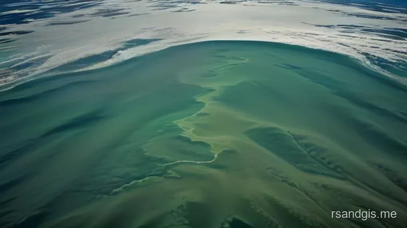
While fractal noise algorithms provide excellent baseline topologies, they fundamentally lack the signature of physical forces—specifically, the erosive power of water. Natural terrains exhibit distinct drainage basins, dendritic river networks, and sediment deposition fans. To synthetically generate these features on a DEM, we must apply hydraulic erosion simulations.

A standard particle-based hydraulic erosion algorithm simulates thousands of discrete water droplets falling onto the DEM grid. Each droplet possesses properties such as water volume, velocity, sediment capacity, and direction. As the droplet traverses the terrain, driven by gravity, it either erodes material from the underlying grid cell or deposits its carried sediment.

The mathematical formulation for a droplet's behavior relies on calculating the surface normal and gradient to determine the flow direction. The steepest descent method (D8 flow routing) checks the 8 neighboring cells to find the maximum elevation drop. The droplet's velocity (\( V \)) is updated based on the local slope angle (\( \alpha \)) and gravity, minus a friction coefficient.

The sediment capacity (\( C \)) of the droplet dictates how much soil it can carry. It is directly proportional to the water volume (\( W \)), the droplet's velocity (\( V \)), and the slope gradient. The relationship is often modeled as:

C = Kc · W · V · sin(α)

Where \( K_c \) is a tunable capacity constant. If the droplet's current sediment load is less than its capacity, it erodes elevation from the DEM and adds it to its load. The erosion amount is a fraction of the difference between capacity and current load, modulated by an erosion rate constant. Conversely, if the load exceeds capacity (which happens when the droplet slows down in flat areas or valleys), it deposits the excess sediment back onto the DEM.

Conceptual Python Implementation: Droplet Erosion

def simulate_hydraulic_erosion(dem, iterations=100000, max_lifetime=30):
    rows, cols = dem.shape
    K_c = 0.1      # Sediment capacity factor
    K_e = 0.05     # Erosion rate
    K_d = 0.05     # Deposition rate
    evap_rate = 0.02
    gravity = 4.0
    
    for _ in range(iterations):
        x, y = np.random.randint(1, rows-2), np.random.randint(1, cols-2)
        water = 1.0
        velocity = 1.0
        sediment = 0.0
        
        for step in range(max_lifetime):
            dx = (dem[x+1, y] - dem[x-1, y]) / 2.0
            dy = (dem[x, y+1] - dem[x, y-1]) / 2.0
            
            length = np.sqrt(dx**2 + dy**2)
            if length == 0:
                break
                
            dir_x, dir_y = -dx/length, -dy/length
            next_x, next_y = x + int(np.round(dir_x)), y + int(np.round(dir_y))
            
            if next_x <= 0 or next_x >= rows-1 or next_y <= 0 or next_y >= cols-1:
                break
                
            delta_h = dem[next_x, next_y] - dem[x, y]
            if delta_h > 0:
                dem[x, y] += sediment
                break
                
            slope = -delta_h
            capacity = max(slope * velocity * water * K_c, 0.01)
            
            if sediment < capacity:
                amount = min((capacity - sediment) * K_e, slope)
                dem[x, y] -= amount
                sediment += amount
            else:
                amount = (sediment - capacity) * K_d
                dem[x, y] += amount
                sediment -= amount
                
            velocity = np.sqrt(velocity**2 + slope * gravity)
            water *= (1 - evap_rate)
            x, y = next_x, next_y
            
    return dem

# Apply erosion
eroded_dem = simulate_hydraulic_erosion(dem_base.copy(), iterations=50000)

3. Example-Based Synthesis and Graph Optimization

While procedural noise and physical simulations are powerful, generating specific terrain types (e.g., karst topography, glacial cirques, or precise geological folds) purely from algorithms can be immensely difficult. Example-based synthesis leverages high-resolution DEMs captured from real-world sensors (such as LiDAR or SRTM data) to guide the generation process.

In patch-based synthesis, an algorithm analyzes a source DEM and extracts localized rectangular patches. When a user provides a macroscopic sketch (e.g., a map indicating ridges and valleys), the algorithm searches the source library for patches that locally match these user-defined features. The challenge lies in stitching these discrete patches together without introducing glaring discontinuities or seams in the elevation data.

To achieve seamless blending, researchers utilize the Poisson equation. Let \( f \) be the unknown scalar height field we wish to synthesize over a domain \( \Omega \), and let \( v \) be a vector field representing the gradient of our assembled source patches. The goal is to find an elevation field \( f \) whose gradient \( \nabla f \) is as close as possible to the guidance vector field \( v \). This is framed as a variational problem, leading to the Poisson equation:

Δf = ∇ · v

Where \( \Delta \) is the Laplace operator and \( \nabla \cdot v \) is the divergence of the guidance field. By setting Dirichlet boundary conditions at the edges of the patches, we can solve this sparse linear system iteratively using techniques like Conjugate Gradient or multigrid methods, resulting in a seamlessly fused terrain that preserves the high-frequency detail of the source patches while adhering to global structural constraints.

4. Modern Horizons: Deep Learning and Diffusion Models

The contemporary frontier of terrain synthesis replaces explicit mathematical modeling with learned representations. Generative Adversarial Networks (GANs) and, more recently, Denoising Diffusion Probabilistic Models (DDPMs) have demonstrated unprecedented capability in generating ultra-realistic DEMs.

A diffusion model operates by taking real DEM data and progressively adding Gaussian noise over a series of time steps until the terrain is reduced to pure noise. A neural network (typically a U-Net architecture) is then trained to reverse this process, predicting the noise added at each step. Once trained, the model can synthesize novel terrains by sampling from a random Gaussian distribution and iteratively denoising it.

These deep learning frameworks implicitly capture complex geomorphological correlations that are incredibly difficult to hard-code, such as the relationship between vegetation cover, soil types, and erosion patterns, provided these features are encoded into multi-channel training tensors alongside the elevation data.

5. Python Ecosystem Prerequisites for DEM Manipulation

To successfully implement the algorithms discussed in this tutorial in a Python environment, several core libraries are strictly required. Understanding their roles is paramount:

• numpy: The fundamental package for scientific computing with Python, used here for representing the continuous DEM scalar field as discrete multidimensional arrays and performing highly optimized, vectorized mathematical operations.
• rasterio: A robust library built on top of the Geospatial Data Abstraction Library (GDAL). It is designed to read and write geospatial raster datasets, bridging the gap between raw numeric arrays and properly georeferenced GIS formats.
• scipy: Often utilized alongside NumPy for more complex spatial operations, such as solving the sparse linear systems generated by Poisson blending or performing multidimensional convolution for smoothing high-frequency artifacts.
• matplotlib: Essential for the immediate two-dimensional rendering and visual debugging of synthesized height maps before they are exported to dedicated GIS suites like ArcGIS or QGIS.

6. DEM Export and I/O with Rasterio

Generating a synthetic NumPy array is only half the battle; to integrate this data into Geographic Information Systems (GIS) like QGIS or ArcGIS, the raw matrix must be properly georeferenced and exported into standard geospatial formats, predominantly GeoTIFF.

When exporting a synthesized DEM, we must define a Coordinate Reference System (CRS) and an affine transform. The affine transform dictates how the 2D grid of pixels maps to real-world coordinates, specifying the spatial resolution (cell size) and the origin point (top-left coordinates).

Conceptual Python Implementation: Exporting to GeoTIFF

import rasterio
from rasterio.transform import from_origin

def export_dem_to_geotiff(dem_array, filename, pixel_size=10.0, origin_lon=0.0, origin_lat=0.0):
    """
    Exports a 2D NumPy array as a georeferenced GeoTIFF.
    
    :param dem_array: 2D numpy array containing elevation data
    :param filename: Output file path
    :param pixel_size: Size of each pixel in meters (assuming projected CRS)
    :param origin_lon: Longitude/Easting of the top-left corner
    :param origin_lat: Latitude/Northing of the top-left corner
    """
    # Define the affine transform
    # from_origin takes (west, north, xsize, ysize)
    transform = from_origin(origin_lon, origin_lat, pixel_size, pixel_size)
    
    # Define the Coordinate Reference System (e.g., EPSG:3857 - Web Mercator)
    crs = rasterio.crs.CRS.from_epsg(3857)
    
    # Open the rasterio dataset in write mode
    with rasterio.open(
        filename,
        'w',
        driver='GTiff',
        height=dem_array.shape[0],
        width=dem_array.shape[1],
        count=1,
        dtype=dem_array.dtype,
        crs=crs,
        transform=transform,
    ) as dataset:
        # Write the DEM array to the first band
        dataset.write(dem_array, 1)

# Export the generated and eroded terrain
# export_dem_to_geotiff(eroded_dem, 'synthetic_terrain_output.tif', pixel_size=30.0)

Conclusion

The synthesis of Digital Elevation Models has evolved from simple mathematical noise functions to highly sophisticated physical simulations and deep learning frameworks. By combining procedural generation algorithms like Fractional Brownian Motion with deterministic hydraulic erosion models, developers and geoscientists can create expansive, highly detailed landscapes that adhere to the physical laws of nature. Furthermore, as example-based and AI-driven methodologies continue to mature, the fidelity of synthetic topographies will become increasingly indistinguishable from real-world geospatial data, unlocking new possibilities across geological modeling, simulation, and digital world-building.