PostGIS Raster Spatial Analysis Tutorial

Table of Contents

• Understanding the Core Concepts of Raster Data in PostGIS
• The Power of Raster Tiling
• The Anatomy and Metadata of a PostGIS Raster
• Installation, Configuration, and Setup
• Spinning Up a PostGIS Database Environment
• Enabling the Necessary Spatial Extensions
• Importing and Ingesting Raster Data into PostGIS
• Mastering the raster2pgsql Utility
• Executing Basic Raster Queries and Extracting Metadata
• Querying and Inspecting Raster Metadata
• Pinpointing and Extracting Specific Pixel Values
• Unleashing Advanced Raster Algebra and Map Algebra
• Executing Single-Band Map Algebra Operations
• Complex Multi-Raster Map Algebra Integration
• Strategic Reclassification of Raster Datasets
• Precision Clipping and Masking Rasters with Vector Data Boundaries
• Mastering the ST_Clip Function
• Elevation Data Analysis: Slope, Aspect, and Hillshade
• Computing Terrain Slope
• Deriving Aspect and Generating Hillshade Visualizations
• Synthesizing Raster and Vector Analytics: Zonal Statistics
• Executing Zonal Statistics: Summarizing Elevation Metrics by Administrative Region
• Critical Performance Tuning and Database Optimization Strategies
• 1. Enforce Tiling Universally
• 2. Rigorously Maintain Spatial Indexes
• 3. Mandate Raster Alignment
• 4. Aggressively Tune PostgreSQL Configuration Parameters
• Troubleshooting Common PostGIS Raster Errors
• Real-world Use Cases and Industry Implementations
• Revolutionizing Precision Agriculture
• Dynamic Flood Risk Modeling and Assessment
• Long-term Climate Data Tracking and Analysis
• Advanced Raster Processing Techniques and Capabilities
• Dynamic ST_Resample and Reprojection Workflows
• Vectorizing Raster Data for Topological Analysis
• Exporting Raster Data for External Visualization
• Conclusion

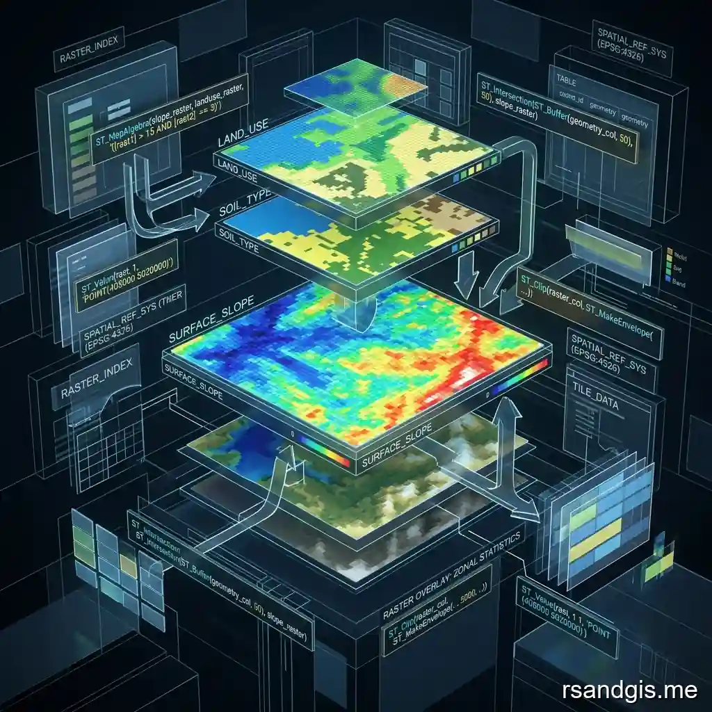
Welcome to this comprehensive postgis raster spatial analysis tutorial. In the rapidly evolving landscape of Geographic Information Systems (GIS) and spatial data management, the ability to process, analyze, and manipulate massive geospatial datasets directly within a relational database management system is not just a luxury; it is an absolute necessity for modern data engineering. PostGIS, the powerful and widely adopted spatial extension for the PostgreSQL database, has long been recognized as the gold standard for handling vector data—such as points, lines, and complex polygons. However, its immense capabilities extend far beyond traditional vector geometries. With the introduction, subsequent maturation, and continuous optimization of the PostGIS Raster extension, users from diverse fields can now natively store, query, modify, and analyze continuous grid-based data structures alongside their traditional vector layers.

These grid structures, commonly referred to as raster datasets, represent some of the most data-intensive formats in the GIS world. They include high-resolution satellite imagery, digital elevation models (DEMs), land cover classifications, climatic temperature grids, and rainfall models. Processing these datasets historically required specialized, expensive, and often cumbersome desktop GIS software. Today, spatial SQL allows you to execute complex remote sensing workflows directly via queries.

This extensive tutorial is meticulously designed to take you on a journey from the very fundamental concepts of raster data architecture within PostGIS to highly advanced spatial analysis techniques. Whether you are an experienced GIS professional looking to transition your local file-based workflows into a scalable database environment, a data scientist exploring spatial datasets for machine learning models, or a backend developer tasked with building high-performance, scalable location-based web applications, mastering PostGIS raster capabilities will exponentially enhance your analytical toolkit. We will cover a vast array of topics, encompassing everything from installation, data ingestion, and structural concepts to map algebra, terrain analysis, performance optimization, workflow automation, and real-world implementation strategies.

Understanding the Core Concepts of Raster Data in PostGIS

Before diving headfirst into SQL queries and practical examples, it is crucially important to understand precisely what raster data is, how it differs fundamentally from vector data, and exactly how the PostGIS architecture handles it internally. A raster is essentially a spatial matrix—a continuous grid of equally sized cells (or pixels) organized into a structured array of rows and columns. Each individual cell within this grid contains a numeric value representing specific geographic information at that exact location on the Earth's surface. This could be continuous data, such as ambient temperature in degrees Celsius or elevation above sea level in meters, or it could be categorical data, such as a land cover class representing "forest," "urban," or "water." Unlike vector data, which relies on mathematical coordinates to define discrete boundaries and shapes, raster data paints a continuous spatial picture.

In the context of PostGIS, the native raster data type empowers you to store this complex grid data directly in database tables. However, a naive approach of storing an entire, massive satellite image (which could easily be several gigabytes in size) in a single database row would be catastrophic for performance. Scanning, reading, and loading a massive image into memory just to query a small neighborhood would be highly inefficient. To solve this, PostGIS utilizes a methodology known as "tiling."

The Power of Raster Tiling

When you ingest a large raster dataset into PostGIS, it is almost always divided into smaller, manageable chunks called tiles (for example, blocks of 100x100 or 256x256 pixels). Each one of these tiles is then stored as an entirely separate row within your database table. This tiling approach, when synergistically combined with PostgreSQL's robust spatial indexing capabilities (specifically GiST indexes), allows the database query planner to perform spatial bounding-box checks. Consequently, PostGIS can instantaneously retrieve only the specific subset of tiles that intersect your specific area of interest, completely ignoring the rest of the massive dataset. This makes localized spatial queries remarkably fast, even when operating on petabytes of imagery.

The Anatomy and Metadata of a PostGIS Raster

A PostGIS raster is not just a blob of pixels; it is a highly structured spatial object that encapsulates critical metadata. Every single raster tile consists of several key structural components that define its spatial reality:

• Spatial Reference System (SRID): The coordinate reference system (CRS) that geographically grounds the raster grid to the real-world Earth surface.
• Scale (Pixel Size): The geographical width and height of each individual pixel in the units of the specified SRID (e.g., a pixel represents 30x30 meters on the ground).
• Skew (Rotation): Parameters defining if the raster grid is rotated relative to the standard North-South / East-West coordinate axes.
• Upper Left Coordinates: The precise real-world X and Y geographical starting point (origin) of the raster grid's top-left corner.
• Width and Height: The specific dimensions of the raster tile, measured in pixels.
• Bands: A raster can be multi-dimensional, containing multiple layers or "bands" of data. For example, a standard color aerial photograph typically contains three distinct bands representing Red, Green, and Blue light. A sophisticated multispectral satellite image might possess ten or more bands, capturing data across various invisible parts of the electromagnetic spectrum, such as near-infrared and thermal infrared.
• Pixel Type: The underlying data type utilized to store the cell values. This is critical for storage optimization and precision. Examples include 8-bit unsigned integers (for simple categorical data or 0-255 color values), 16-bit integers, or 32-bit floating-point numbers (crucial for precise continuous data like elevation).
• NoData Value: A specialized, designated numeric value utilized to explicitly represent the absence of valid data for a particular pixel (e.g., -9999).

Installation, Configuration, and Setup

To embark on our spatial analysis journey, you absolutely must have access to a working PostgreSQL database with the PostGIS extension properly installed and configured. Fortunately, modern iterations of PostGIS include comprehensive raster support bundled by default. If you are starting fresh and want a hassle-free, reproducible environment, the absolute easiest and most recommended way to get up and running is leveraging containerization technology, specifically using the official PostGIS Docker image.

Spinning Up a PostGIS Database Environment

Ensure you have Docker installed on your system. Open your terminal or command prompt and execute the following command to download and initiate a robust PostgreSQL instance equipped with PostGIS:

docker run --name postgis-tutorial -e POSTGRES_PASSWORD=mysecretpassword -p 5432:5432 -d postgis/postgis:15-3.3

This command launches a container running PostgreSQL version 15 with PostGIS 3.3, exposes the standard port 5432, and sets a secure default password. Once the container spins up successfully, you need to connect to it. You can use command-line clients like psql, or graphical user interfaces such as pgAdmin, DBeaver, or QGIS. Once connected as the postgres superuser, create an isolated, dedicated database for your analytical projects:

CREATE DATABASE raster_analysis_db;
\c raster_analysis_db;

Enabling the Necessary Spatial Extensions

Simply creating the database is not enough. You must explicitly instruct PostgreSQL to load and enable the spatial functions and data types provided by PostGIS within your newly created database. Execute the following standard SQL commands:

CREATE EXTENSION postgis;
CREATE EXTENSION postgis_raster;

It is vital to verify that the extensions were installed, activated, and are functioning correctly. You can easily validate your environment by checking the installed PostGIS version utilizing a built-in function:

SELECT postgis_full_version();

Carefully inspect the output string. If you prominently see both POSTGIS and POSTGIS_RASTER listed, your database environment is successfully primed and ready to ingest and manipulate complex spatial grid data.

Importing and Ingesting Raster Data into PostGIS

Transitioning raw raster files from your local filesystem into the relational database is the crucial first practical step in your workflow. The PostGIS ecosystem provides a remarkably powerful, flexible, and robust command-line executable utility specifically engineered for this task: raster2pgsql. This application leverages the industry-standard Geospatial Data Abstraction Library (GDAL) under the hood. Consequently, it can seamlessly read virtually any standard raster format imaginable—including GeoTIFF, JPEG2000, PNG, NetCDF, and ERDAS Imagine—and systematically translates them into raw SQL CREATE TABLE and INSERT statements.

Mastering the raster2pgsql Utility

Let us construct a practical scenario. Assume you possess a high-resolution Digital Elevation Model (DEM) stored as a GeoTIFF file on your hard drive, named seattle_elevation_model.tif. Your objective is to load this data into a new database table logically named dem_data. You would navigate to the directory containing your file in your terminal and execute a command pipeline similar to this:

raster2pgsql -s 4326 -I -C -M -t 100x100 seattle_elevation_model.tif public.dem_data > dem_import_script.sql
psql -h localhost -U postgres -d raster_analysis_db -f dem_import_script.sql

This pipeline is the standard best practice for raster ingestion. Let us dissect and completely demystify the critical flags utilized in the raster2pgsql command:

• -s 4326: This explicitly defines the Spatial Reference System Identifier (SRID) of the source data. In this common example, 4326 corresponds to the standard WGS 84 coordinate system (longitude/latitude). Ensuring the correct SRID is paramount for accurate spatial relationships later.
• -I: This is arguably the most important flag for performance. It instructs the utility to automatically generate a GiST (Generalized Search Tree) spatial index on the resulting raster geometry column. Without this index, your spatial queries will resort to excruciatingly slow sequential table scans.
• -C: This flag applies a comprehensive set of standard raster constraints to the newly created table. These constraints act as rigorous data integrity checks, ensuring that all tiles loaded into the table strictly share the exact same SRID, pixel resolution (scale), spatial alignment, NoData values, and band structure. This is required for many raster functions to operate correctly.
• -M: This flag intelligently appends a VACUUM ANALYZE command to the end of the generated SQL script. Executing this immediately after the massive data insertion optimizes the PostgreSQL query planner's internal statistics, ensuring it constructs the most efficient query plans possible from the very beginning.
• -t 100x100: This dictates the tiling dimensions. Instead of loading the image as one monolithic block, it chops the raster into a grid of tiles, each measuring exactly 100 pixels wide by 100 pixels high. We discussed the critical importance of this earlier.

Executing Basic Raster Queries and Extracting Metadata

Once your massive raster datasets are safely and structurally ingested into PostGIS, you can commence querying the database to extract vital metadata, validate the ingestion, and perform basic preliminary inspections. The PostGIS Raster Application Programming Interface (API) provides a vast suite of functions specifically tailored for this purpose. You will notice that all spatial functions are prefixed with ST_, signifying Spatial Type.

Querying and Inspecting Raster Metadata

To fully understand the inherent physical properties and structure of your imported raster, you can leverage functions such as ST_Width, ST_Height, ST_SRID, and ST_BandPixelType. Because our table design utilizes tiling and contains thousands of rows (where each row represents a distinct tile), we typically append a LIMIT 1 clause to our query to inspect the metadata of just a single tile. We can safely make the assumption that the -C constraints flag we used during import guarantees consistency across all other tiles in the table.

SELECT 
    ST_Width(rast) AS tile_width_pixels,
    ST_Height(rast) AS tile_height_pixels,
    ST_SRID(rast) AS coordinate_system_srid,
    ST_NumBands(rast) AS total_band_count,
    ST_BandPixelType(rast, 1) AS datatype_of_band_1,
    ST_ScaleX(rast) AS horizontal_pixel_size,
    ST_ScaleY(rast) AS vertical_pixel_size
FROM dem_data 
LIMIT 1;

Pinpointing and Extracting Specific Pixel Values

One of the most frequent foundational requirements in spatial analysis is determining the precise numeric value of a raster dataset at a specific, known geographic coordinate. For instance, you might urgently need to find the exact elevation above sea level at a specific GPS point defined by its longitude and latitude. To achieve this, you construct a PostGIS vector point geometry, utilize a spatial intersection to rapidly locate the specific raster tile containing that point, and finally extract the underlying pixel value.

SELECT 
    ST_Value(rast, 1, ST_SetSRID(ST_MakePoint(-122.3321, 47.6062), 4326)) AS precise_elevation_at_point
FROM dem_data
WHERE ST_Intersects(rast, ST_SetSRID(ST_MakePoint(-122.3321, 47.6062), 4326));

In this elegant query, the ST_Value function is responsible for reaching into band 1 of the raster and pulling out the numerical value exactly at the specified point geometry. Crucially, the WHERE ST_Intersects(...) clause ensures that the database engine utilizes the GiST spatial index. It aggressively filters the table, ensuring that the computationally expensive ST_Value function is only executed on the single specific tile that physically covers that exact coordinate, guaranteeing lightning-fast response times even on tables with millions of tiles.

Unleashing Advanced Raster Algebra and Map Algebra

The true, unparalleled power of conducting PostGIS raster spatial analysis is fully realized through the application of Map Algebra. Map algebra is a profound analytical framework that involves systematically applying complex mathematical operations, statistical functions, or conditional logical statements to one or more overlapping raster grids, thereby dynamically generating an entirely new, derivative raster output. PostGIS handles this incredible capability elegantly and efficiently using the highly versatile ST_MapAlgebra suite of functions.

Executing Single-Band Map Algebra Operations

Let us consider a highly practical scenario. Suppose you have successfully imported a digital elevation model (DEM) where the elevation values natively represent meters. However, the stakeholders for your current project strictly require all elevation metrics to be reported and visualized in feet. You can effortlessly utilize ST_MapAlgebra to iterate through the entire grid and multiply every single pixel value by the conversion factor of 3.28084.

CREATE TABLE dem_data_feet AS
SELECT 
    rid,
    ST_MapAlgebra(
        rast, 1, 
        '32BF', 
        '[rast] * 3.28084'
    ) AS rast
FROM dem_data;

Let us deeply analyze this command. The '32BF' argument explicitly defines the desired pixel type of the newly generated output raster. In this case, it signifies a 32-bit floating-point number, which is necessary to preserve the decimal precision resulting from the multiplication. The core of the operation is the algebraic expression string: '[rast] * 3.28084'. PostGIS evaluates this expression for every individual pixel in the source dataset. The query ultimately creates a completely new, spatially indexed, and correctly tiled raster dataset table containing the newly converted values, all while keeping the heavy processing entirely within the database server.

Complex Multi-Raster Map Algebra Integration

The analytical capabilities of Map Algebra expand exponentially when you begin combining multiple, distinct raster datasets. A classic, widely utilized example in remote sensing and environmental monitoring is the calculation of the Normalized Difference Vegetation Index (NDVI). NDVI is derived from satellite imagery by comparing the reflectance values of the Red and Near-Infrared (NIR) light bands. The standard mathematical formula for NDVI is strictly defined as (NIR - Red) / (NIR + Red).

Assuming you have populated a table named landsat_imagery containing multispectral satellite data, where you know that band 3 represents the Red spectrum and band 4 represents the NIR spectrum, you can compute NDVI directly using spatial SQL:

CREATE TABLE vegetation_health_ndvi AS
SELECT 
    rid,
    ST_MapAlgebra(
        rast, 4, -- Targeting the NIR band
        rast, 3, -- Targeting the Red band
        '([rast1] - [rast2]) / ([rast1] + [rast2])::float', 
        '32BF'
    ) AS rast
FROM landsat_imagery;

This sophisticated query processes the two distinct bands cell-by-cell in a highly optimized, simultaneous manner, dynamically generating a new continuous raster surface that quantitatively represents vegetation health and density. Executing this massive calculation within the robust PostgreSQL engine allows you to easily parallelize the operations across multiple CPU cores and keeps the processing intimately close to where the data is stored, completely eradicating the costly overhead of exporting gigabytes of raw data to external, standalone desktop software for processing.

Strategic Reclassification of Raster Datasets

Reclassification is a fundamental spatial operation involving the systematic replacement of existing continuous or discrete pixel values with completely new values based on explicitly defined ranges, thresholds, or logical conditions. This technique is absolutely essential for transforming complex, continuous data (like precise elevation metrics or exact temperatures) into simplified, categorical data that is easier to interpret (like categorizing a landscape into "low," "medium," and "high" flood risk zones based on specific elevation thresholds).

PostGIS offers the highly efficient ST_Reclass function designed exactly for this purpose. Suppose we have a requirement to rigorously categorize our continuous elevation model into three specific, discrete topographical zones for a regional planning study:

• Elevations from 0 to 500 meters → Reclassify as Value 1 (Designated Lowland)
• Elevations from 500 to 1500 meters → Reclassify as Value 2 (Designated Midland)
• Elevations from 1500 to 9000 meters → Reclassify as Value 3 (Designated Highland)

CREATE TABLE topographical_zones AS
SELECT 
    rid,
    ST_Reclass(
        rast, 1, 
        '0-500:1, 500-1500:2, 1500-9000:3', 
        '8BUI', 
        0
    ) AS rast
FROM dem_data;

The core intelligence of this query lies in the reclassification string: '0-500:1, 500-1500:2, 1500-9000:3'. This string acts as a translation dictionary, defining the strict rules for conversion. Furthermore, the resulting raster intelligently uses an 8-bit unsigned integer pixel type ('8BUI'). Because the newly generated dataset only needs to store the simple integer values 1, 2, and 3, using an 8-bit integer saves an enormous amount of physical storage space and memory overhead compared to retaining the original, heavy 32-bit floating-point data structure used for the raw DEM.

Precision Clipping and Masking Rasters with Vector Data Boundaries

One of the most profound and celebrated advantages of utilizing PostGIS for spatial analysis is the completely seamless, native interoperability between disparate vector and raster data types within the same query environment. During analytical workflows, you will frequently encounter the strict requirement to restrict, limit, or "clip" your continuous raster analysis to a very specific geographical boundary precisely defined by a vector polygon. This process is ubiquitously known in GIS terminology as clipping or masking.

Mastering the ST_Clip Function

Imagine a scenario where your database houses a comprehensive table named municipal_boundaries, containing highly detailed vector polygons for various cities. Your immediate objective is to extract the continuous elevation model strictly within the exact, irregular city limits of "Seattle", discarding everything outside. You accomplish this cleanly and efficiently using the ST_Clip function joined with a spatial intersection.

CREATE TABLE seattle_specific_dem AS
SELECT 
    m.city_name,
    ST_Clip(r.rast, m.geom) AS clipped_elevation_raster
FROM dem_data AS r
JOIN municipal_boundaries AS m
ON ST_Intersects(r.rast, m.geom)
WHERE m.city_name = 'Seattle';

The powerful ST_Clip function acts as a digital cookie-cutter. It literally slices the intersecting raster tiles perfectly along the intricate, jagged borders of the provided vector geometry. Any raster pixels that physically fall outside the boundaries of the polygon, yet remain within the square bounds of the intersecting tile, are immediately nullified and set to the raster's designated NoData value. This process is highly optimized, reduces the dataset to only the relevant pixels, and perfectly prepares the spatial data for highly localized, hyper-focused statistical analysis or visualization.

Elevation Data Analysis: Slope, Aspect, and Hillshade

If your spatial workflows heavily involve working with Digital Elevation Models (DEMs), you will be thrilled to discover that PostGIS natively provides a suite of highly optimized, built-in functions specifically tailored for complex terrain analysis. This completely removes the tedious and error-prone requirement for developers to manually write complex, multi-cell map algebra expressions to derive standard topographical metrics.

Computing Terrain Slope

Slope represents the mathematical rate of change of elevation across the surface, essentially quantifying the steepness of the terrain. Identifying steep slopes is critical for landslide risk modeling, road construction planning, and hydrological flow analysis. To seamlessly calculate a slope raster surface from a base DEM, you utilize the ST_Slope function.

CREATE TABLE regional_slope_raster AS
SELECT 
    rid,
    ST_Slope(rast, 1, '32BF', 'DEGREES', 1.0) AS rast
FROM dem_data;

This SQL command processes the DEM and elegantly calculates the slope output in degrees. The crucial parameter 1.0 represents the scale factor (often referred to as the Z-factor). This factor is absolutely critical to understand and configure correctly if your horizontal spatial units (for example, decimal degrees in a WGS84 projection) differ fundamentally from your vertical units (for example, elevation stored in meters). It is highly and universally recommended as a GIS best practice to project your base DEM into an appropriate local projected coordinate system (such as UTM) where both the horizontal and vertical units are identical (e.g., both in meters) before executing advanced terrain algorithms to avoid severe distortion.

Deriving Aspect and Generating Hillshade Visualizations

Similarly to slope, you can effortlessly calculate the Aspect (which indicates the specific compass direction that a slope physically faces, crucial for solar radiation modeling and vegetation distribution analysis) and Hillshade (which generates a stunning 3D shaded relief map, incredibly useful for basemap visualization and cartographic output).

-- Calculate the Aspect (Facing direction)
CREATE TABLE regional_aspect_raster AS
SELECT 
    rid, 
    ST_Aspect(rast, 1, '32BF', 'DEGREES', true) AS rast 
FROM dem_data;

-- Calculate a Cartographic Hillshade
CREATE TABLE regional_hillshade_raster AS
SELECT 
    rid, 
    ST_HillShade(rast, 1, '32BF', 315.0, 45.0, 255.0, 1.0, false) AS rast 
FROM dem_data;

The highly configurable ST_HillShade function grants you granular control over the virtual lighting environment. It allows you to explicitly specify the azimuth (the compass direction, set to 315.0 degrees here representing the North-West) and altitude (the angle above the horizon, set to 45.0 degrees) of a virtual sun, providing a highly customizable, beautiful rendering of the underlying terrain topology.

Synthesizing Raster and Vector Analytics: Zonal Statistics

Comprehensive spatial analysis frequently culminates in the requirement to summarize massive amounts of continuous raster data by grouping it within discrete vector boundaries—a process universally referred to in the geospatial industry as Zonal Statistics. PostGIS handles this complex requirement elegantly and natively through aggregate functions, most notably ST_SummaryStats.

Executing Zonal Statistics: Summarizing Elevation Metrics by Administrative Region

Suppose you are tasked with a critical analysis where you must definitively find the minimum, maximum, and average (mean) elevation for every single administrative county residing in your database. This requires a complex orchestration of spatial operations: you must strategically join the raster table with the vector polygon table, accurately clip the raster grids to the exact irregular boundaries of the polygons, mathematically union the fragments, and then finally calculate the descriptive statistics on the resulting isolated pixels.

SELECT 
    c.county_name,
    (ST_SummaryStats(ST_Union(ST_Clip(r.rast, c.geom)))).min AS absolute_min_elevation,
    (ST_SummaryStats(ST_Union(ST_Clip(r.rast, c.geom)))).max AS absolute_max_elevation,
    (ST_SummaryStats(ST_Union(ST_Clip(r.rast, c.geom)))).mean AS calculated_avg_elevation
FROM dem_data AS r
JOIN administrative_counties AS c
ON ST_Intersects(r.rast, c.geom)
GROUP BY c.county_name;

Do not underestimate the sheer power of this query. It performs a highly complex, computationally intensive orchestration of spatial algorithms behind the scenes. It aggressively finds only the spatially intersecting raster tiles, surgically clips them to the intricate county boundaries, mathematically merges (unions) those clipped, fragmented tiles into a unified, seamless raster object per county, and finally computes the detailed statistical summary. While this operation is admittedly resource-intensive on the database server, executing this massive calculation entirely within the database fundamentally avoids the crippling network bottleneck of transferring gigabytes of raw raster and vector data across the wire to external application servers.

Critical Performance Tuning and Database Optimization Strategies

Working with vast, high-resolution raster datasets within a relational database architecture is inherently memory and CPU-intensive. To absolutely ensure that your spatial queries remain highly performant and do not crash your database, you must aggressively adopt and implement several critical best practices specific to PostGIS Raster administration.

1. Enforce Tiling Universally

As emphatically stated during the import section, you must never, under any circumstances, store an entire high-resolution image in a single database row. Optimal tile sizes generally range from 50x50 to 256x256 pixels, heavily depending on your specific query patterns. Smaller tiles generate more rows, but they allow for incredibly fine-grained spatial index bounding-box lookups, minimizing the amount of irrelevant data loaded into active memory during processing.

2. Rigorously Maintain Spatial Indexes

You must meticulously ensure that a GiST index is consistently present and healthy on every raster geometry column in your database. Furthermore, if you execute a map algebra operation or a complex query that generates a brand new physical table, you must explicitly create a new GiST index manually on that new table before querying it further.

CREATE INDEX optimal_new_raster_idx ON newly_created_raster_table USING GIST (ST_ConvexHull(rast));

3. Mandate Raster Alignment

When you attempt to perform map algebra or complex mathematical operations between two fundamentally different raster datasets (for example, attempting to subtract a historic temperature grid from a modern temperature grid), they MUST be perfectly aligned. Alignment strictly means they mathematically share the exact same SRID, pixel resolution (scale), and precise grid snapping on the X and Y axes. If they are misaligned, your queries will fail or produce garbage data. If they are not natively aligned, you are required to use the ST_Resample function to strategically warp, rubber-sheet, or interpolate one raster grid to perfectly match the strict mathematical grid of the other before performing any algebra.

4. Aggressively Tune PostgreSQL Configuration Parameters

Heavy raster processing relies extraordinarily heavily on available system RAM. You must manually intervene and tune your primary postgresql.conf configuration file. Significantly increase the parameters for shared_buffers, work_mem, and especially maintenance_work_mem to properly accommodate massive in-memory array processing and complex spatial joins. Furthermore, you should explicitly enable and tune parallel query processing (specifically altering max_parallel_workers_per_gather) to aggressively leverage modern multi-core server processors when your database is tasked with scanning and evaluating millions of individual raster tiles.

Troubleshooting Common PostGIS Raster Errors

Working with spatial databases often presents unique challenges. When performing complex operations, you might encounter specific errors. One of the most common is the "Rasters do not have the same alignment" error during Map Algebra. This strictly means your grids do not line up pixel-for-pixel. You must resolve this using ST_Resample or ST_SnapToGrid to align the secondary raster to the primary raster's spatial footprint.

Another frequent issue is out-of-memory (OOM) errors during heavy ST_Union operations. If you attempt to union thousands of high-resolution tiles simultaneously without adequate RAM or proper tiling strategies, PostgreSQL will terminate the query to protect system stability. The solution is always to ensure your tiles are small, limit your queries using strict bounding boxes, and utilize temporary tables to break down massive union operations into smaller, digestible chunks.

Real-world Use Cases and Industry Implementations

To fully contextualize the immense capabilities and value of PostGIS raster technology, let us examine a few detailed, real-world scenarios across various industries where this specific technology architecture shines brilliantly.

Revolutionizing Precision Agriculture

Modern agronomists and agricultural analysts aggressively use PostGIS to manage massive influxes of drone imagery and multi-temporal satellite data. By storing multi-spectral continuous rasters in the database, they can compute complex vegetation indices (like NDVI, EVI, or SAVI) on the fly for thousands of specific, irregularly shaped farm field boundaries (stored as vector polygons). This architecture allows for the rapid development of automated alerting systems. When crop health metrics mathematically fall below historical rolling averages in highly specific spatial zones, the database can trigger automated workflows for targeted, hyper-local interventions, drastically reducing chemical usage and optimizing overall yield.

Dynamic Flood Risk Modeling and Assessment

Urban planners and emergency management agencies integrate high-precision Digital Elevation Models directly with vector representations of complex river networks and civil infrastructure. By leveraging in-database map algebra and terrain analysis, they can dynamically simulate rapidly rising water levels. They can write and execute queries that programmatically determine: "If regional water levels rise by exactly 2.5 meters, immediately identify and flag all residential building footprints (vectors) that physically intersect with raster pixels whose calculated elevation strictly falls below the newly established flood plane." This provides instantaneous, database-driven, highly accurate risk assessments crucial for insurance modeling, zoning, and emergency evacuation planning.

Long-term Climate Data Tracking and Analysis

Climate scientists frequently process massive NetCDF climate models—which are inherently multi-dimensional, temporal raster grids—by programmatically loading them into PostGIS arrays. They can then perform highly complex, database-native time-series analysis. For example, they can effortlessly calculate the absolute average temperature change over a rolling fifty-year decade for highly specific, complex ecological regions by executing massive zonal statistics queries across hundreds of related raster tables, each representing different distinct time slices.

Advanced Raster Processing Techniques and Capabilities

As you gain proficiency and grow more comfortable with the foundational basics, you can confidently begin to explore the outer, more advanced limits of PostGIS raster capabilities.

Dynamic ST_Resample and Reprojection Workflows

You can programmatically and dynamically alter the fundamental resolution or the overarching coordinate projection of a raster grid using ST_Resample or ST_Transform. For instance, if you are required to rapidly downsample a massive, high-resolution 1-meter aerial ortho-photograph into a more manageable 10-meter resolution for a low-bandwidth regional web mapping overview, ST_Resample allows you to execute this while explicitly choosing advanced interpolation algorithms like Nearest Neighbor (for categorical data), Bilinear, or Cubic convolution (for continuous imagery) to ensure data integrity during the transformation.

Vectorizing Raster Data for Topological Analysis

Conversely, sometimes your analytical workflow requires you to go in the opposite direction—converting continuous grid data into discrete vector polygons. The ST_DumpAsPolygons function is explicitly designed for this. It takes a categorical raster dataset (such as a complex land-cover classification map derived from machine learning) and programmatically generates a distinct, discrete vector polygon for every single contiguous patch of identical pixel values. This is an incredibly powerful and useful tool for dynamically generating highly accurate vector boundaries of natural features like forests, agricultural plots, or water bodies directly from classified remote sensing imagery.

SELECT 
    (ST_DumpAsPolygons(rast)).geom AS extracted_vector_polygon,
    (ST_DumpAsPolygons(rast)).val AS specific_land_cover_class
FROM classified_land_cover_raster;

Exporting Raster Data for External Visualization

After successfully completing your complex, in-database spatial analysis, you will frequently need to extract the resulting derivative raster datasets out of the database architecture. This is necessary for final cartographic visualization in desktop GIS software like QGIS or ArcGIS Pro, or for serving the data to the web via mapping servers like GeoServer or MapServer. PostGIS provides highly efficient, native export functions that seamlessly convert the internal tiled database representation back into standard, universally recognized file formats.

The ST_AsTIFF, ST_AsJPEG, and ST_AsPNG functions explicitly allow you to serialize the raster data structures. Because your data is highly tiled within the database for performance, you typically must strategically use ST_Union to mathematically merge the disparate tiles back together into a single cohesive image before invoking the export function.

SELECT 
    ST_AsTIFF(ST_Union(rast), 'LZW') AS compressed_tiff_binary_output
FROM seattle_specific_dem;

This powerful query directly produces a binary bytea output stream representing a complete, fully formed, and LZW-compressed GeoTIFF file. You can effortlessly pipe this binary output directly to a physical file on your filesystem using the PostgreSQL psql copy command, or by utilizing standard binary data handling techniques within your application's programming language driver (such as Python's psycopg2 or Node.js's pg module).

Conclusion

Mastering comprehensive raster analysis natively within PostGIS opens an incredibly powerful, transformative new paradigm for modern geospatial data engineering and architecture. By decisively moving the complex processing logic deep into the database itself—as close as physically possible to where the massive datasets actually reside—you completely eliminate the severe network bottlenecks and extreme latency associated with traditional file-based I/O and heavily fragmented desktop analytical workflows. Throughout this extensive guide, you have learned the critical fundamental principles of how to expertly import, efficiently query, mathematically manipulate, and thoroughly analyze continuous surface data using robust, standard spatial SQL constructs.

While this deep-dive tutorial extensively covers a very significant breadth of core functionality, the larger PostGIS ecosystem is vast, deeply mature, and continually improving with every release. By creatively and strategically combining the powerful raster techniques learned here today with traditional vector analysis, complex network routing (via pgRouting), and massive point-cloud processing capabilities, you can architect and build truly enterprise-grade spatial applications capable of efficiently solving the most complex geographic problems at a global scale. Embrace the unmatched power of spatial SQL, experiment relentlessly with your own diverse datasets, and continue aggressively pushing the boundaries of what is technically possible within your modern database architecture.