Deep Learning Based Point Cloud Classification Using PDAL

Image Processing August 18, 2026

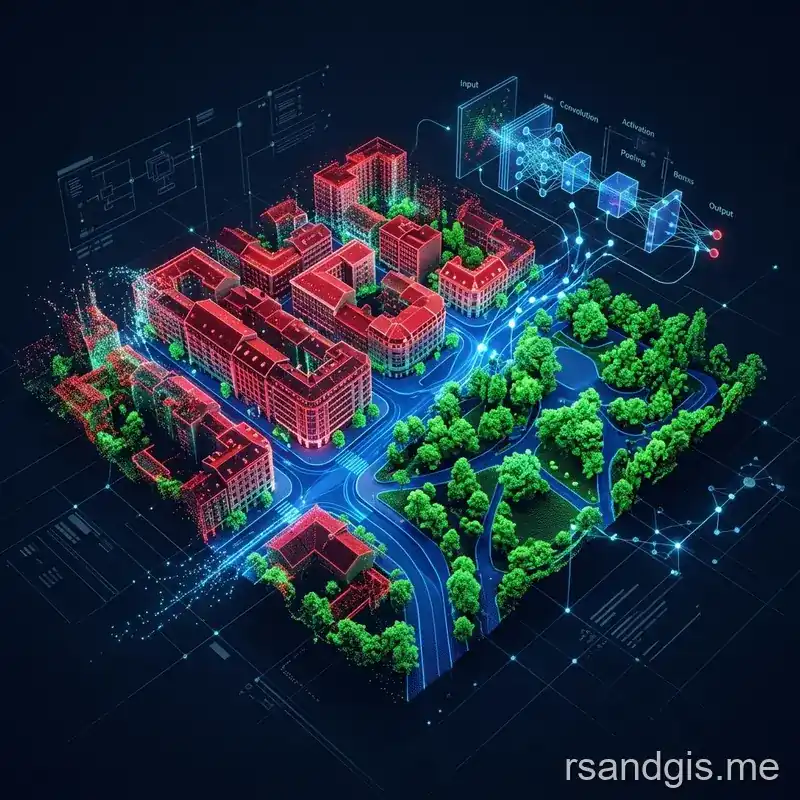
In recent years, the geospatial industry has witnessed a paradigm shift with the integration of artificial intelligence into spatial analysis. One of the most significant breakthroughs in this domain is deep learning based point cloud classification using pdal. As LiDAR sensors become more ubiquitous—spanning airborne, terrestrial, and mobile mapping systems—they generate massive volumes of unstructured 3D data. The need for robust, scalable, and automated processing pipelines has never been more urgent. By combining the powerful data manipulation capabilities of the Point Data Abstraction Library (PDAL) with cutting-edge neural networks, practitioners can seamlessly transform raw, noisy laser scans into highly structured, semantically rich datasets. This article delves deep into the technical workflow required to operationalize this integration, offering a comprehensive guide from raw data ingestion to advanced model deployment.

The Anatomy of LiDAR and the Point Cloud Challenge

Light Detection and Ranging (LiDAR) technology captures the physical world with remarkable precision, producing point clouds that consist of millions, if not billions, of discrete data points in three-dimensional space. Each point inherently possesses X, Y, and Z coordinates, but often includes additional attributes such as intensity, return number, number of returns, scan angle, and sometimes even RGB values acquired from co-registered imagery. While this wealth of information is invaluable for applications ranging from autonomous driving to forestry management, it presents significant computational challenges.

Unlike 2D images, which are structured as dense, regular grids of pixels, point clouds are fundamentally unstructured and sparse. The density of points varies based on the distance from the sensor, occlusions, and the reflective properties of the scanned surfaces. This irregular data structure makes traditional convolutional neural networks (CNNs) unsuitable without heavy modifications. Furthermore, the sheer volume of data involved in a typical survey can overwhelm even the most robust computing architectures. Processing a single tile of urban LiDAR data requires efficient memory management and optimized spatial indexing to query local neighborhoods rapidly.

To overcome these hurdles, researchers have historically relied on handcrafted features—such as planarity, linearity, and surface roughness—combined with classical machine learning algorithms like Random Forests or Support Vector Machines (SVMs). However, these methods often struggle to generalize across different environments and sensor types. The transition to deep learning has promised autonomous feature extraction and superior accuracy, but it necessitates a seamless conduit between the raw data and the algorithmic frameworks. This is precisely where PDAL proves its worth.

In addition to algorithmic hurdles, the geospatial characteristics of point clouds require specialized handling. Because LiDAR coordinates are usually referenced to a global coordinate system, the raw values are extraordinarily large numbers. Feeding such massive coordinate values directly into a neural network results in vanishing or exploding gradients during backpropagation. This requires meticulous data standardization and local coordinate normalization, an operation that must be consistently applied during both training and real-time inference to ensure accurate predictions.

Why Choose PDAL for Data Abstraction?

The Point Data Abstraction Library (PDAL) is a C++ open-source library and suite of tools designed specifically for translating and processing point cloud data. Much like its counterpart GDAL (Geospatial Data Abstraction Library) does for raster and vector data, PDAL provides an abstraction layer that allows users to interact with numerous point cloud formats (such as LAS, LAZ, BPF, EPT, and ASCII) through a unified interface. Its architecture is built around the concept of pipelines—a sequential chain of readers, filters, and writers that stream data efficiently.

Using PDAL offers several distinct advantages in the context of machine learning workflows. Firstly, its declarative JSON-based pipeline syntax enables reproducible and easily automatable data processing tasks. Instead of writing monolithic scripts, developers can chain modular operations, such as spatial clipping, coordinate reprojection, and attribute filtering. Secondly, PDAL's robust set of filters includes advanced algorithms for ground classification (like the Simple Morphological Filter, SMRF, or the Progressive Morphological Filter, PMF), outlier removal, and voxel-based decimation.

Crucially, PDAL provides native bindings for Python, which serves as the lingua franca of the modern deep learning ecosystem. By utilizing the pdal Python package, data scientists can execute complex pipelines within a Python script and extract the results directly into Numpy arrays. This eliminates intermediate disk I/O operations, significantly accelerating the data preparation phase and bridging the gap between geospatial data engineering and AI model training.

Moreover, the extensible nature of PDAL permits developers to inject their own logic through Python filters directly within the pipeline. This tight coupling means that a deep learning model trained in PyTorch or TensorFlow can be invoked dynamically within a PDAL stream, enabling on-the-fly classification and writing the predicted labels immediately back to standard LiDAR formats without cumbersome intermediate parsing steps.

Navigating the Deep Learning Landscape for 3D Data

Before diving into the implementation, it is essential to understand the architectural paradigms that dominate 3D deep learning. Because raw point clouds do not conform to a regular grid, researchers have developed three primary strategies to process them: voxelization, projection, and direct point processing.

Voxel-based Methods: These techniques partition the 3D space into a regular grid of volumetric pixels (voxels). Each voxel aggregates the properties of the points it encapsulates. Once the data is voxelized, 3D Convolutional Neural Networks (3D CNNs) can be applied. Models like VoxelNet and MinkowskiNet have shown great success with this approach. The primary drawback is the computational cost; increasing the grid resolution leads to a cubic increase in memory consumption, often resulting in sparse, inefficient tensors.

Projection-based Methods: Another approach involves projecting the 3D point cloud onto multiple 2D planes (multi-view) or into spherical coordinates (such as range images for autonomous driving LiDAR). Standard 2D CNNs can then process these projections. While this reduces the dimensionality and leverages highly optimized 2D architectures, it inherently loses some topological and geometric information during the projection process.

Point-based Methods: Pioneered by the seminal PointNet architecture, these methods consume raw point clouds directly. PointNet utilizes multi-layer perceptrons (MLPs) applied independently to each point, combined with a symmetric pooling function (typically Max Pooling) to achieve permutation invariance. Its successor, PointNet++, introduces hierarchical feature learning by partitioning the point set into overlapping local regions. More recent architectures, such as RandLA-Net, employ random sampling and advanced local feature aggregation to scale efficiently to massive point clouds. Graph Convolutional Networks (GCNs) like DGCNN represent another powerful point-based approach, constructing dynamic graphs to capture local geometric relationships.

For most modern aerial and terrestrial LiDAR classification tasks, point-based methods have emerged as the dominant architecture due to their ability to ingest raw geometric features directly without the lossy transformation steps required by voxelization or planar projection. Consequently, this workflow focuses on interfacing PDAL directly with point-based neural network models.

Step 1: The Preprocessing Pipeline – Preparing Data with PDAL

The foundation of any successful deep learning project is high-quality data. In the realm of point clouds, this means standardizing the dataset, removing noise, and extracting relevant features. PDAL pipelines are uniquely suited for these tasks. Below, we outline a typical PDAL JSON pipeline designed to prepare a raw LAS file for neural network ingestion.

{
  "pipeline": [
    {
      "type": "readers.las",
      "filename": "raw_survey.las"
    },
    {
      "type": "filters.elm"
    },
    {
      "type": "filters.outlier",
      "method": "statistical",
      "mean_k": 8,
      "multiplier": 3.0
    },
    {
      "type": "filters.smrf",
      "ignore": "Classification[7:7]"
    },
    {
      "type": "filters.hag_nn"
    },
    {
      "type": "filters.voxeldownsize",
      "cell": 0.1
    },
    {
      "type": "writers.las",
      "filename": "processed_survey.las",
      "extra_dims": "all"
    }
  ]
}

Let us dissect this pipeline step by step:

• Data Ingestion: The readers.las stage efficiently streams the raw LiDAR data into memory.
• Noise and Outlier Removal: The filters.elm (Extended Local Minimum) identifies low noise points, while the filters.outlier utilizes statistical outlier removal. It computes the mean distance to the 8 nearest neighbors (mean_k) and flags points whose distance exceeds the global mean plus 3 standard deviations (multiplier). This step is critical because deep learning models are sensitive to anomalous spatial artifacts that can distort local feature extraction.
• Ground Classification: The filters.smrf applies the Simple Morphological Filter to classify ground points (class 2). Distinguishing the ground topography is vital for contextualizing above-ground objects like buildings and trees. The network learns spatial relationships much better when it explicitly knows the ground datum.
• Height Above Ground (HAG) Normalization: Raw Z-coordinates reflect absolute elevation above sea level, which varies geographically. The filters.hag_nn computes the relative height of each point above the nearest ground point. Normalizing the Z-axis ensures that a 10-meter tree looks identical to the network regardless of whether it grows at sea level or in a mountainous region.
• Downsampling: High-density point clouds can exhaust GPU memory. The filters.voxeldownsize stage applies a voxel grid filter, retaining only a single representative point within each 10cm cubic cell. This balances computational feasibility with sufficient geometric detail required for semantic segmentation.

Step 2: Bridging the Gap – Integrating PDAL with Python and PyTorch

With the preprocessing logic defined, the next stage is to bridge PDAL and the Python deep learning ecosystem. By embedding the pipeline execution directly within Python, we can generate training batches dynamically without writing intermediate files to disk. This in-memory transition is paramount for reducing storage overhead and expediting the data loading lifecycle during model training.

import pdal
import numpy as np
import torch
from torch.utils.data import Dataset, DataLoader

class PointCloudDataset(Dataset):
    def __init__(self, file_list, pipeline_json):
        self.file_list = file_list
        self.pipeline_json = pipeline_json
        
    def __len__(self):
        return len(self.file_list)
        
    def __getitem__(self, idx):
        file_path = self.file_list[idx]
        
        # Inject the file path dynamically into a basic pipeline
        pipeline_def = f"""
        {{
          "pipeline": [
            "{file_path}",
            {{
              "type": "filters.hag_nn"
            }}
          ]
        }}
        """
        
        pipeline = pdal.Pipeline(pipeline_def)
        pipeline.execute()
        
        # Extract Numpy array
        arr = pipeline.arrays[0]
        
        # Extract specific features: X, Y, Height Above Ground, Intensity
        features = np.vstack((arr['X'], arr['Y'], arr['HeightAboveGround'], arr['Intensity'])).transpose()
        labels = arr['Classification']
        
        # Center the X and Y coordinates around the origin
        features[:, 0] -= np.mean(features[:, 0])
        features[:, 1] -= np.mean(features[:, 1])
        
        # Convert to PyTorch tensors
        features_tensor = torch.tensor(features, dtype=torch.float32)
        labels_tensor = torch.tensor(labels, dtype=torch.long)
        
        return features_tensor, labels_tensor

This custom Dataset class encapsulates the data ingestion logic beautifully. It leverages the PDAL Python API to execute a pipeline on the fly, fetch the structured Numpy array, and extract only the necessary dimensions. Spatial normalization (centering the X and Y coordinates) is performed to ensure numerical stability during neural network training and prevent the model from memorizing absolute geographic locations. The resulting PyTorch tensors are subsequently ready for batching and shuffling via a standard DataLoader.

Step 3: Architecting and Training the Neural Network

For this workflow, we will outline a PointNet-inspired architecture, although frameworks like PyTorch Geometric offer robust implementations of more advanced models like PointNet++ and DGCNN out of the box. The core principle of point-based architectures relies on learning independent point features and aggregating them using symmetric functions.

A simplified implementation of a point feature extractor in PyTorch involves a series of 1D convolutions acting on the point dimensions. Because point clouds are strictly unordered sets, standard 2D convolutions applied in image processing cannot be directly utilized. Instead, 1D convolutions (acting as shared Multi-Layer Perceptrons) process each point identically and independently.

import torch.nn as nn
import torch.nn.functional as F

class PointNetClassifier(nn.Module):
    def __init__(self, num_classes, num_features=4):
        super(PointNetClassifier, self).__init__()
        # Shared MLPs for feature extraction
        self.conv1 = nn.Conv1d(num_features, 64, 1)
        self.conv2 = nn.Conv1d(64, 128, 1)
        self.conv3 = nn.Conv1d(128, 1024, 1)
        
        # Batch Normalization layers
        self.bn1 = nn.BatchNorm1d(64)
        self.bn2 = nn.BatchNorm1d(128)
        self.bn3 = nn.BatchNorm1d(1024)
        
        # MLPs for classification
        self.fc1 = nn.Linear(1024, 512)
        self.fc2 = nn.Linear(512, 256)
        self.fc3 = nn.Linear(256, num_classes)
        
        self.dropout = nn.Dropout(p=0.3)
        self.bn4 = nn.BatchNorm1d(512)
        self.bn5 = nn.BatchNorm1d(256)

    def forward(self, x):
        # Input shape: [Batch_Size, Num_Features, Num_Points]
        num_points = x.size(2)
        
        # Local feature extraction
        x = F.relu(self.bn1(self.conv1(x)))
        x = F.relu(self.bn2(self.conv2(x)))
        x = F.relu(self.bn3(self.conv3(x)))
        
        # Global Feature Aggregation via Max Pooling
        x = torch.max(x, 2, keepdim=True)[0]
        x = x.view(-1, 1024)
        
        # Classification head
        x = F.relu(self.bn4(self.fc1(x)))
        x = F.relu(self.bn5(self.fc2(x)))
        x = self.dropout(x)
        x = self.fc3(x)
        
        return F.log_softmax(x, dim=1)

Training this network requires the strategic selection of an appropriate loss function. For semantic segmentation (assigning a class label to every individual point) or patch-based classification, Cross-Entropy Loss is the standard baseline. However, LiDAR point cloud datasets suffer inherently from extreme class imbalance. For instance, the sheer volume of ground and vegetation points vastly outweighs the sparse representations of streetlights, fire hydrants, or pedestrians. To mitigate this pervasive issue, practitioners should employ Weighted Cross-Entropy or Focal Loss algorithms, which dynamically penalize the misclassifications of minority classes far more severely than dominant background classes.

During the training loop, the optimizer (typically Adam or the more modern AdamW variant) updates the network weights iteratively. A learning rate scheduler (such as Cosine Annealing) is highly recommended to anneal the learning rate smoothly as the model converges toward the local minima. The definitive evaluation metric of choice in 3D semantic segmentation is the mean Intersection over Union (mIoU), which provides a significantly more robust performance measure than overall accuracy, especially given the aforementioned class imbalance that heavily skews accuracy percentages.

Step 4: Inference and Post-Processing – Completing the Cycle

Once the model is rigorously trained, validated, and optimized, it must be deployed for inference on entirely unlabelled production datasets. The true power of PDAL shines brilliantly in this deployment phase, as we can inject our trained PyTorch model directly back into a PDAL pipeline utilizing the versatile filters.python capability. This methodology allows PDAL to read a designated chunk of points, effortlessly pass them to an external Python function that executes the PyTorch model inference, and seamlessly write the newly predicted classification labels back into the structured point cloud file.

First, we define a dedicated Python script (e.g., inference.py) containing the distinct function to be invoked by the PDAL framework:

import numpy as np
import torch
from model import PointNetClassifier

# Load the trained model globally to avoid reloading per chunk
device = torch.device("cuda" if torch.cuda.is_available() else "cpu")
model = PointNetClassifier(num_classes=5).to(device)
model.load_state_dict(torch.load("best_model.pth"))
model.eval()

def predict_chunk(ins, outs):
    # 'ins' is a dictionary of input Numpy arrays provided by PDAL
    X = ins['X']
    Y = ins['Y']
    Z = ins['Z']
    Intensity = ins['Intensity']
    
    # Feature engineering (e.g., local centering)
    cx = X - np.mean(X)
    cy = Y - np.mean(Y)
    
    # Stack and format for PyTorch: [Batch, Channels, Points]
    features = np.vstack((cx, cy, Z, Intensity)).astype(np.float32)
    features_tensor = torch.tensor(features).unsqueeze(0).to(device)
    
    with torch.no_grad():
        predictions = model(features_tensor)
        predicted_classes = torch.argmax(predictions, dim=1).cpu().numpy().flatten()
        
    # 'outs' is a dictionary where we pass the modified arrays back to PDAL
    outs['Classification'] = predicted_classes
    return True

With this Python integration script fully prepared, we can seamlessly construct the final PDAL JSON execution pipeline to process large, complex geographic tiles iteratively using a filters.splitter or processing spatial chunks directly:

{
  "pipeline": [
    {
      "type": "readers.las",
      "filename": "unclassified_data.las"
    },
    {
      "type": "filters.python",
      "module": "inference",
      "function": "predict_chunk",
      "add_dimension": "Classification"
    },
    {
      "type": "writers.las",
      "filename": "classified_output.las"
    }
  ]
}

This streamlined, closed-loop integration ensures that the complex tensor operations required for AI inference are safely abstracted away from the end-user. The pipeline can be efficiently executed via the standard PDAL command-line interface, embedded into C++ applications, or deployed extensively in a serverless cloud computing environment to process massive, city-scale datasets concurrently without manual intervention.

Real-World Case Study: Urban Infrastructure Mapping

To tangibly contextualize this intricate workflow, consider a large-scale municipal project aimed at mapping urban infrastructure—specifically identifying buildings, utility poles, and tree canopies—for an ambitious smart city digital twin initiative. Traditional classification routines utilized in older software rely heavily on rigid geometric thresholds. A utility pole, for example, might be identified by searching for vertical, cylindrical clusters of points. However, in dense, chaotic urban environments, the physical geometries of utility poles, traffic lights, and thin tree trunks often overlap significantly, inevitably causing unacceptably high false-positive rates when using classical rule-based filtering methodologies.

By implementing the robust deep learning workflow discussed above, the municipality can transcend the stringent limitations of hard-coded heuristic rules. The workflow begins by strictly utilizing PDAL to normalize the height of the urban survey data and geometrically segment it into overlapping 20-meter by 20-meter spatial tiles. This meticulous tiling strategy critically ensures that the point density remains easily manageable for standard GPU memory limits without causing hardware bottlenecks.

A DGCNN (Dynamic Graph CNN) architecture is thoughtfully chosen for its superior ability to capture fine-grained local geometric structures, which is fundamentally critical for distinguishing the intricate branching patterns of trees from the rigid, artificial structures of power lines and utility poles. The network is carefully trained on a meticulously manually labeled subset of the city's LiDAR data, aggressively utilizing data augmentation techniques such as random rotation, point scaling, and Gaussian jittering to substantially improve the model's robustness against varying point densities and inherent sensor noise profiles.

Upon finally reaching statistical convergence, the extensively trained DGCNN is elegantly wrapped in the PDAL filters.python module. The immense city-scale dataset, comprising terabytes of raw LAZ files, is strategically distributed across a high-performance cloud computing cluster. The PDAL pipelines execute seamlessly in parallel, continuously fetching tiles, running the DGCNN AI inference, and immediately appending the newly derived classification labels. The breathtaking result is a highly accurate, flawlessly semantically segmented 3D structural map of the entire city. Subsequent post-processing steps—again executed flawlessly via PDAL pipelines—can rapidly filter the dataset to isolate specific infrastructural classes. For instance, an automated pipeline can instantly extract all points classified mathematically as "Utility Pole", mathematically apply a clustering algorithm like DBSCAN, and precisely calculate the exact geographic centroid of each cluster to automatically generate an actionable GIS shapefile of pole locations for maintenance crews.

Overcoming Common Challenges: Memory Management and Edge Cases

When practically implementing this highly technical workflow in a demanding production environment, data engineers inevitably encounter several complex practical challenges. Chief among these persistent issues is the strict management of GPU memory resources. Unlike standardized image datasets where the structural dimensions are strictly uniform, LiDAR point clouds exhibit radically variable point densities. A fixed spatial bounding box located in a dense urban center might contain upwards of two million points, while the exact same sized volumetric box in a sparsely populated rural area might contain only ten thousand points. Ingesting two million points directly into a modern neural network will almost certainly instantly trigger a catastrophic Out-Of-Memory (OOM) error.

To effectively mitigate this dangerous inconsistency, the PyTorch data loader must absolutely employ dynamic, geometry-aware sampling strategies. Farthest Point Sampling (FPS) is universally acknowledged and widely used to iteratively downsample a highly variable point cloud to a strict, fixed number of data points (e.g., 4096 or 8192 points) while remarkably preserving the underlying holistic geometry. While computationally significantly more expensive than naive random sampling, FPS practically guarantees that the critical structural integrity of the objects is fully maintained. In Python workflows, effectively utilizing specialized libraries like PyTorch3D or Open3D substantially accelerates the mathematically intense FPS algorithm through highly optimized custom CUDA kernels.

Another major structural hurdle is dealing proactively with boundary effects or edge artifacts. When a large point cloud is systematically tiled for inference, massive objects that lie directly on the artificial boundary of two distinct tiles are arbitrarily split. A residential building sliced perfectly in half might not possess the necessary geometric context for the neural network to classify it correctly, ultimately leading to embarrassing misclassifications directly along the tile seams. The industry-standard solution to this spatial problem is to deliberately implement spatially overlapping inference grids. By computing the deep learning predictions on heavily overlapping spatial tiles and subsequently employing a sophisticated mathematical consensus mechanism—such as simple majority voting or distance-weighted probability averaging—for the points residing purely in the overlap region, the nasty seam artifacts are effectively and beautifully smoothed out, yielding a completely seamless, structurally homogenous classification map across the entire vast survey area.

Optimization and Advanced Deployment Strategies

As corporate organizations aggressively scale their AI-driven LiDAR classification workflows, sheer computational efficiency rapidly becomes a primary operational bottleneck. Deep learning models, particularly intricate graph-based architectures, are notoriously intensely compute-hungry. Therefore, meticulously optimizing the trained neural model for scalable deployment is frankly just as important as the lengthy training phase itself.

One of the absolute most effective technical strategies is exporting the fully trained PyTorch model directly to the Open Neural Network Exchange (ONNX) universal format. ONNX powerfully provides a universally standard representation for deep learning models, allowing them to be subsequently executed using fiercely highly optimized runtime engines like ONNX Runtime or the proprietary NVIDIA TensorRT framework. TensorRT aggressively performs neural layer fusion, precision calibration (e.g., smoothly converting FP32 weights to faster FP16 or INT8 formats), and highly dynamic memory management, remarkably resulting in total inference speeds up to 5x to 10x faster than native, unoptimized PyTorch execution.

Integrating an ultra-fast ONNX/TensorRT model into the previously discussed PDAL Python filter explicitly follows the exact same architectural logic as demonstrated previously, but effectively substitutes the heavy PyTorch execution context for an incredibly lightweight ONNX Runtime session. This seemingly minor structural change drastically reduces operational latency, ultimately enabling true near real-time point cloud classification for bleeding-edge applications like autonomous navigation processing or immediate post-flight drone surveys where time is incredibly critical.

Furthermore, managing large-scale spatial indexing efficiently is absolutely crucial for cloud operations. While PDAL beautifully provides robust tools for splitting and tiling, aggressively employing heavily specialized point cloud databases like Entwine or PostgreSQL deeply integrated with the Pointcloud extension can vastly improve large-scale data retrieval times. By intelligently structuring the data in a hierarchical, spatially-indexed format (e.g., EPT - Entwine Point Tile format), remote inference pipelines can mathematically query specific geographic extents and required resolutions dynamically, strictly only processing data at the exact required level of detail without unnecessarily reading entire raw LAS files into volatile memory.

Conclusion and Future Trajectories

The strategic technical integration of the Point Data Abstraction Library with advanced, high-performance neural network frameworks undeniably represents a phenomenal quantum leap in geospatial data processing. The beautifully automated, highly robust nature of modern deep learning definitively overcomes the inherent fragility of traditional, heuristic-based filtering algorithms, while PDAL's elegantly declarative JSON pipelines flawlessly handle the profound complexities of point cloud ingestion, geometric normalization, and spatial export.

This deeply technical workflow—comprehensively ranging from initial structural filtering and volumetric voxelization to custom PyTorch Dataset creation and closed-loop, large-scale inference—immensely empowers modern data scientists and GIS professionals to confidently tackle formerly completely insurmountable computational challenges in 3D spatial analysis. The robust automation of comprehensive urban infrastructure mapping, highly advanced autonomous vehicle environment perception, and massive large-scale forestry inventory are merely the beginning of this technological revolution.

Looking aggressively ahead, the rapid evolution of this powerful methodology will almost certainly likely be shaped by the meteoric rise of sophisticated Transformer architectures specifically adapted for 3D spatial data, such as Point Transformer, which mathematically promise even greater classification accuracies by intelligently leveraging complex self-attention mechanisms to perfectly capture long-range contextual relationships within the chaotic point cloud. Additionally, incredible advancements in hardware edge computing will undoubtedly see PDAL and heavily optimized deep learning models rapidly deployed directly on active LiDAR sensors or embedded UAV companion computers, ultimately enabling true real-time, on-the-fly analytics precisely at the point of data capture. As the overwhelming volume of global 3D spatial data continues its staggering exponential growth trajectory, flawlessly mastering this specific intersection of robust data abstraction and cutting-edge artificial intelligence will fundamentally remain an absolutely essential, highly sought-after skillset for the modern, elite spatial data engineer.

Frequently Asked Questions