Advanced PyQGIS Workflows: Integrating Machine Learning Models for Raster Prediction

Introduction to PyQGIS and Machine Learning

The intersection of Geographic Information Systems (GIS) and artificial intelligence represents the most significant paradigm shift in spatial analytics over the past decade. While traditional GIS workflows rely on deterministic tools and manual rule-based classification, modern geospatial architectures demand predictive capabilities, autonomous data processing, and scalable machine learning (ML) models. QGIS, through its powerful Python API (PyQGIS), serves as the ultimate bridge between traditional spatial data infrastructure (SDI) and the modern Python data science ecosystem. The ability to write Python code that directly manipulates QGIS memory layers, interfaces with GDAL, and simultaneously feeds data into Scikit-Learn or TensorFlow is unprecedented.

In this comprehensive masterclass, we will explore advanced methodologies for integrating state-of-the-art machine learning libraries—specifically Scikit-Learn and TensorFlow—directly into PyQGIS environments. We will move beyond simple point-and-click operations to construct fully autonomous, headless geospatial ETL (Extract, Transform, Load) pipelines capable of processing terabytes of raster imagery, extracting spectral signatures, training predictive land-cover classification models, and automatically rendering the output back into the QGIS map canvas.

By the conclusion of this tutorial, you will have engineered a complete end-to-end predictive pipeline that treats QGIS not merely as a desktop application, but as a spatial compute engine. This is particularly crucial for organizations dealing with high-frequency satellite data, such as PlanetScope or Sentinel-2, where manual digitization is physically impossible.

Machine learning in GIS is not just about prediction; it's about automation, accuracy, and scaling. Traditional GIS analysts spend countless hours digitizing polygons. By leveraging PyQGIS and Scikit-Learn, we can train a model on a small subset of digitized polygons and instantly classify millions of pixels across an entire satellite scene with higher accuracy and consistency than human operators.

The Architectural Framework: PyQGIS as a Headless Engine

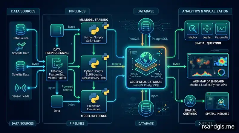
Before diving into machine learning code, it is critical to understand the execution context of PyQGIS. PyQGIS can be executed in three primary modes: within the QGIS Python Console, as a QGIS Plugin, or as a standalone headless script. For enterprise machine learning pipelines, the headless approach is paramount.

Headless PyQGIS allows you to bypass the Graphical User Interface (GUI), allocating 100% of your machine's CPU and RAM to mathematical computation. This is essential when working with massive raster arrays that require intense memory buffering during model inference. The GUI overhead of rendering millions of vertices or pixel values can easily crash a machine learning pipeline before it even reaches the training phase.

Furthermore, running headless allows you to deploy your PyQGIS scripts inside Docker containers, AWS EC2 instances, or Kubernetes clusters. This is the foundation of modern WebGIS and Cloud-Native geospatial processing. You are no longer limited by the RAM of your local workstation; you can scale your compute horizontally.

Setting Up the Standalone Environment

To execute PyQGIS alongside data science libraries, you must ensure your Python environment path is correctly configured to locate the qgis.core modules while also having access to scikit-learn, numpy, pandas, and geopandas.

Setting up the OSGeo4W shell or a Conda environment is usually the best approach. You must map the QGIS prefix path so that the standalone script can locate the core libraries, providers, and plugins. Failure to set the prefix path correctly will result in segmentation faults or missing provider errors when trying to load vector or raster layers.

# Initializing a Headless PyQGIS Environment
import sys
import os
from qgis.core import QgsApplication, QgsVectorLayer, QgsRasterLayer, QgsProject

# Supply path to qgis install location (Windows OSGeo4W example)
QgsApplication.setPrefixPath(r"C:\OSGeo4W\apps\qgis", True)

# Create a reference to the QgsApplication
# Setting the second argument to False disables the GUI
qgs = QgsApplication([], False)
qgs.initQgis()

print("QGIS Engine Successfully Initialized in Headless Mode.")
# Your machine learning pipeline will execute here
# ...
# Finally, exit QGIS cleanly
qgs.exitQgis()

Once the QgsApplication is running in headless mode, you have access to the entirety of the QGIS processing framework (including GDAL, SAGA, and GRASS algorithms) without ever opening a window. This is the exact architecture used by massive geospatial companies to process daily satellite ingests.

Data Preparation: Extracting Raster Features for ML

Machine learning models require structured tabular data (2D arrays of features and targets), whereas GIS data is inherently spatial (multi-dimensional raster grids and vector geometries). The most complex aspect of integrating ML with PyQGIS is the ETL process: flattening spatial datasets into feature matrices.

In traditional machine learning, you might load a CSV file using Pandas. In GeoAI, your "CSV" is a multi-gigabyte GeoTIFF file, and your "rows" are individual pixels. Your "columns" (features) are the spectral bands of that pixel (Red, Green, Blue, Near-Infrared, SWIR, etc.).

Reading Multispectral Imagery via QgsRasterLayer

Consider a scenario where we have a multispectral Sentinel-2 raster image containing 10 spectral bands, alongside a vector shapefile containing training polygons (e.g., regions manually labeled as Forest, Water, Urban, and Agriculture). We must extract the spectral values (features) for every single pixel that falls strictly inside these training polygons.

This process is known as "Zonal Extraction" or "Raster Masking". While QGIS has built-in Zonal Statistics tools, they are often too slow for machine learning pipelines that require extracting millions of pixels. Instead, we use PyQGIS to read the geometry bounds, and then use GDAL's Python bindings to read the raw NumPy arrays directly from disk.

from qgis.analysis import QgsZonalStatistics
import numpy as np
from osgeo import gdal, ogr, osr

def extract_raster_features(raster_path, vector_path):
    raster_layer = QgsRasterLayer(raster_path, "Sentinel2_Image")
    vector_layer = QgsVectorLayer(vector_path, "Training_Data", "ogr")
    
    if not raster_layer.isValid() or not vector_layer.isValid():
        raise Exception("Layer failed to load!")
        
    features = []
    labels = []
    
    # Open dataset using GDAL for high-speed array reading
    dataset = gdal.Open(raster_path)
    transform = dataset.GetGeoTransform()
    
    # Iterate through training polygons
    for feature in vector_layer.getFeatures():
        geom = feature.geometry()
        label = feature['class_id']
        
        # In a production environment, we use rasterio or gdal.RasterizeLayer 
        # to create a binary mask of the polygon, then extract the pixels
        # where the mask == 1.
        
        # For demonstration, assume we extract a NumPy array of spectral signatures
        # pixel_signatures shape: (N_pixels, N_bands)
        # pixel_signatures = extract_pixels_in_geom(dataset, geom, transform)
        
        # features.append(pixel_signatures)
        # labels.extend([label] * len(pixel_signatures))
        
    # return np.vstack(features), np.array(labels)
    pass

The output of this function is a massive 2D NumPy array (X) where every row is a pixel and every column is a spectral band, and a 1D NumPy array (Y) containing the corresponding integer class ID for that pixel. We have successfully bridged the gap between GIS and Data Science.

Feature Engineering for Geospatial Data

Raw spectral bands are rarely enough to achieve state-of-the-art accuracy. Machine learning models thrive on engineered features. In the context of remote sensing, feature engineering involves calculating spectral indices (like NDVI, NDWI, or SAVI) and appending them as new columns in our feature matrix.

PyQGIS makes this incredibly easy because we are already working with NumPy arrays. For example, to calculate the Normalized Difference Vegetation Index (NDWI), we simply perform array mathematics on the Near-Infrared and Red bands.

# Assuming X is a numpy array where column 3 is RED and column 7 is NIR
red_band = X[:, 3]
nir_band = X[:, 7]

# Calculate NDVI: (NIR - RED) / (NIR + RED)
# Add a small epsilon to avoid division by zero
epsilon = 1e-8
ndvi = (nir_band - red_band) / (nir_band + red_band + epsilon)

# Append NDVI as a new feature column
X_engineered = np.column_stack((X, ndvi))
print(f"Original shape: {X.shape}, New shape: {X_engineered.shape}")

Beyond spectral indices, spatial features can also be engineered. Texture metrics (like Grey Level Co-occurrence Matrix - GLCM), elevation data from a Digital Elevation Model (DEM), or slope/aspect derivatives can all be flattened into 1D arrays and appended to our feature matrix. The more relevant geospatial context we provide to the model, the higher its predictive accuracy.

Training the Predictive Model with Scikit-Learn

Once the spatial data is structured into NumPy arrays, the GIS context temporarily vanishes, and pure data science takes over. For land cover classification based on spectral signatures, ensemble learning algorithms like Random Forests (RF), Support Vector Machines (SVM), or Gradient Boosting Machines (XGBoost/LightGBM) are industry standards.

Random Forests are particularly favored in the remote sensing community due to their robustness against overfitting, their ability to handle high-dimensional feature spaces without feature selection, and their interpretability (we can easily extract feature importances to see which spectral bands contributed most to the classification).

Furthermore, Random Forests are highly parallelizable. We can set n_jobs=-1 in Scikit-Learn to utilize every CPU core on our headless server, drastically reducing training time for massive datasets.

from sklearn.ensemble import RandomForestClassifier
from sklearn.model_selection import train_test_split
from sklearn.metrics import classification_report, accuracy_score, confusion_matrix
import joblib
import seaborn as sns
import matplotlib.pyplot as plt

# X represents the engineered spectral bands, Y represents the land cover class IDs
# Split data into training (70%) and validation (30%) sets
X_train, X_test, y_train, y_test = train_test_split(X_engineered, y, test_size=0.3, random_state=42)

# Initialize the Random Forest Classifier
# class_weight='balanced' ensures rare classes (like small water bodies) aren't ignored
rf_model = RandomForestClassifier(n_estimators=500, max_depth=30, n_jobs=-1, class_weight='balanced')

# Train the model
print("Training Random Forest Classifier on Spatial Features...")
rf_model.fit(X_train, y_train)

# Evaluate the model
predictions = rf_model.predict(X_test)
print("Model Accuracy:", accuracy_score(y_test, predictions))
print("\nDetailed Classification Report:")
print(classification_report(y_test, predictions))

# Persist the model to disk for future inference without retraining
joblib.dump(rf_model, 'land_cover_rf_model.pkl')
print("Model successfully saved to disk.")

Model Inference and Re-Spatialization

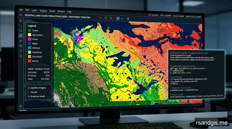
The final and most visually rewarding phase of the PyQGIS machine learning pipeline is inference. We must feed the entire extent of our input raster into the trained Scikit-Learn model, predict the class of every single pixel, and then—crucially—reconstruct a brand new geospatial raster layer from the resulting 1D array of predictions.

This is where many data scientists stumble. They can predict the arrays, but they don't know how to inject those arrays back into a valid GeoTIFF with the correct spatial reference system (SRS), affine geotransform, and NoData values. GDAL is the industry standard tool for this.

Generating the Prediction Raster

To reconstruct the spatial reference system, bounding box, and pixel resolution, we use GDAL to clone the metadata from the original Sentinel-2 image. The output is a single-band thematic raster where pixel values correspond to predicted land cover classes (e.g., 1=Water, 2=Forest, 3=Urban).

Because satellite images are massive (often billions of pixels), we cannot load the entire image into RAM for prediction. We must read the image in chunks (or blocks), predict the chunk, and write the chunk to the output file.

def predict_and_export_raster_chunked(input_raster, model_path, output_raster):
    # Load the trained Scikit-Learn model
    model = joblib.load(model_path)
    
    # Open input imagery
    src_ds = gdal.Open(input_raster)
    bands = src_ds.RasterCount
    cols = src_ds.RasterXSize
    rows = src_ds.RasterYSize
    
    # Create the output geospatial raster
    driver = gdal.GetDriverByName('GTiff')
    out_ds = driver.Create(output_raster, cols, rows, 1, gdal.GDT_Byte)
    out_ds.SetGeoTransform(src_ds.GetGeoTransform())
    out_ds.SetProjection(src_ds.GetProjection())
    out_band = out_ds.GetRasterBand(1)
    out_band.SetNoDataValue(0)
    
    # Process in chunks of 1024x1024 pixels to save RAM
    chunk_size = 1024
    
    for y in range(0, rows, chunk_size):
        for x in range(0, cols, chunk_size):
            # Calculate actual chunk size (handling edge cases)
            y_size = min(chunk_size, rows - y)
            x_size = min(chunk_size, cols - x)
            
            # Read chunk across all bands
            chunk_data = np.zeros((y_size, x_size, bands))
            for b in range(bands):
                chunk_data[:, :, b] = src_ds.GetRasterBand(b+1).ReadAsArray(x, y, x_size, y_size)
                
            # Flatten chunk to 2D
            reshaped_chunk = chunk_data.reshape((y_size * x_size, bands))
            
            # Feature Engineering for the chunk (e.g., NDVI)
            # ...
            
            # Predict
            predictions_1d = model.predict(reshaped_chunk)
            
            # Reshape back to 2D raster chunk
            prediction_2d = predictions_1d.reshape((y_size, x_size))
            
            # Write to output file
            out_band.WriteArray(prediction_2d, x, y)
            
    out_band.FlushCache()
    print(f"Successfully generated predictive raster: {output_raster}")

# Execute the chunked inference
# predict_and_export_raster_chunked('sentinel2_clip.tif', 'land_cover_rf_model.pkl', 'predicted_landcover.tif')

Automating the Workflow with Apache Airflow

While running these scripts manually on a workstation is powerful, enterprise GIS architectures require automation. You don't want a human executing a Python script every time the European Space Agency uploads a new Sentinel-2 tile. By integrating PyQGIS scripts into Apache Airflow Directed Acyclic Graphs (DAGs), organizations can orchestrate autonomous ETL pipelines that trigger automatically.

Airflow allows you to define tasks—such as Download_Sentinel_Imagery, Extract_Features, Train_Random_Forest, and Generate_Predictive_Map—and execute them in a strict dependency sequence. If a task fails (e.g., the ESA API goes down), Airflow handles retries and alerting automatically.

Furthermore, because our PyQGIS script is entirely headless, it can be containerized using Docker. Each Airflow task can spin up an isolated Docker container, inject the new satellite imagery, run the PyQGIS machine learning pipeline, save the resulting GeoTIFF to an Amazon S3 bucket, and spin down. This allows for infinite scalability. If 100 satellite images arrive on the same day, Airflow spins up 100 PyQGIS containers in parallel.

Advanced Topic: Deep Learning with TensorFlow in QGIS

While Random Forests operate on individual pixel values, Deep Learning models—specifically Convolutional Neural Networks (CNNs)—operate on spatial context (patches of pixels). This allows CNNs to recognize shapes, edges, and textures, making them infinitely superior for tasks like automated building footprint extraction or road network tracing.

Integrating TensorFlow or PyTorch with PyQGIS is fundamentally similar to the Scikit-Learn workflow, but the ETL phase is vastly more complex. Instead of extracting 1D pixel arrays, we must use PyQGIS and GDAL to slice our massive raster into thousands of smaller 256x256 pixel image chips. These chips are then fed into a U-Net or Mask R-CNN architecture for semantic segmentation.

The resulting predictions are 256x256 binary masks, which must be stitched back together into a massive global raster using GDAL, and then polygonized using gdal.Polygonize() or PyQGIS native tools to generate final vector shapefiles.

Conclusion: The Future of Spatial Computing

The integration of PyQGIS with modern machine learning libraries transforms QGIS from a traditional mapping interface into a high-performance spatial analytics engine. By mastering headless execution, array manipulation with GDAL and NumPy, and predictive modeling with Scikit-Learn, geospatial developers can architect automated pipelines that vastly outperform manual digitization.

As spatial data volumes continue to explode due to high-revisit satellite constellations, drone fleets, and IoT sensor networks, the era of clicking buttons in a GUI is rapidly coming to an end. The ability to rapidly train, deploy, and execute automated machine learning models using Python will become the defining skill of the next-generation GIS professional. Embrace the code, leverage the algorithms, and turn your QGIS environment into a predictive powerhouse.