object-based image analysis vs pixel-based classification in gee

Image Processing August 18, 2026

Welcome to this comprehensive and deep technical dive into the world of remote sensing, geospatial analytics, and Earth observation. In this extensively detailed article, we will thoroughly explore the ongoing debate and practical implementations surrounding object-based image analysis vs pixel-based classification in gee. If you are a geospatial analyst, a remote sensing scientist, a geographer, or an enthusiast working with massive datasets, you have undoubtedly encountered the formidable challenge of choosing the optimal classification approach for your mapping projects. The decision between analyzing individual, isolated pixels or segmenting images into meaningful, contiguous objects is a foundational one that dictates your overall accuracy, computational efficiency, and workflow design within the Google Earth Engine (GEE) environment. Over the course of this extensive guide, we will break down the mechanics, algorithms, limitations, and advanced workarounds for both methodologies.

Introduction to Image Classification in Remote Sensing

Image classification forms the absolute core of remote sensing applications. It is the computational process of categorizing all pixels in a digital image into one of several distinct land cover classes or thematic categories. This categorized data is then used to produce thematic maps, such as land use and land cover (LULC) maps, deforestation tracking datasets, urban expansion visualizations, and agricultural yield predictions. Historically, remote sensing scientists have relied almost exclusively on pixel-based approaches because early satellite imagery (like the early Landsat missions, which featured 30-meter to 60-meter spatial resolution) possessed moderate to coarse spatial resolutions. In these older, foundational datasets, individual pixels often represented a diverse mixture of different features on the ground, but the pixels were large enough that analyzing them individually made logical and computational sense given the hardware limitations of the era.

However, as satellite sensor technology rapidly advanced and high-resolution imagery from commercial platforms like Sentinel-2, PlanetScope, WorldView, and uncrewed aerial vehicles (UAVs) became ubiquitous and cost-effective, the analytical paradigm shifted dramatically. Suddenly, a single tree crown, a residential house roof, or a small vehicle was no longer represented by a single mixed pixel, but rather by dozens or even hundreds of pure, high-resolution pixels. Applying traditional pixel-based classification algorithms to these ultra-high-resolution datasets often resulted in chaotic, "speckled," and highly noisy maps that were difficult to interpret and functionally useless for precise zoning or counting. This necessity birthed Object-Based Image Analysis (OBIA), a method that intelligently groups similar adjacent pixels into objects before classifying them. Today, implementing these techniques in cloud platforms like Google Earth Engine presents a unique set of advantages, challenges, and computational hurdles that require a deep understanding of distributed computing.

Understanding Pixel-Based Classification

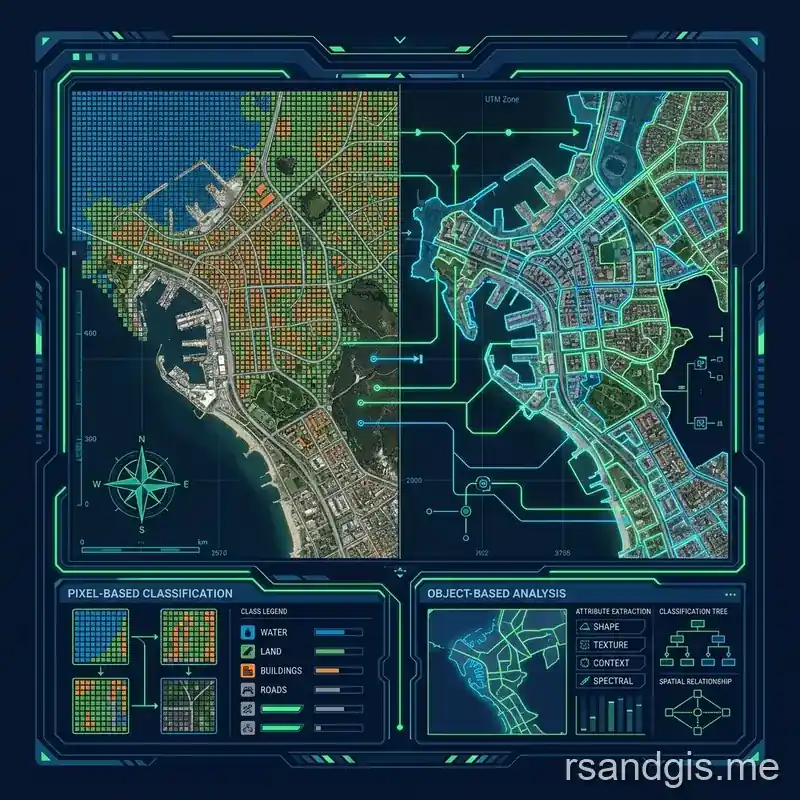
Pixel-based classification analyzes each pixel in an image completely independently, based solely on its individual spectral signature—the unique way a surface reflects or absorbs electromagnetic radiation across various specific wavelengths (bands) of the electromagnetic spectrum. The fundamental, underlying assumption of pixel-based classification is that every thematic class has a distinct, statistically separable spectral response. For example, if a water body absorbs near-infrared light entirely while healthy vegetation reflects it strongly, the classification algorithm can easily differentiate between a "water" pixel and a "vegetation" pixel simply by looking at their numerical values in those specific near-infrared bands, without any regard for where the pixel is located spatially.

In the Google Earth Engine environment, pixel-based classification is incredibly popular, widely taught, and heavily utilized because it aligns perfectly with GEE's inherent distributed processing architecture. GEE distributes processing across thousands of Google servers by dividing the world into small, discrete map tiles and processing the pixels within those tiles in parallel. Because pixel-based algorithms do not need to "know" what adjacent pixels are doing, they are inherently parallelizable. They scale almost infinitely without running into the memory bottlenecks that plague more complex spatial algorithms. You can easily train a Random Forest (RF), Support Vector Machine (SVM), or Classification and Regression Tree (CART) model on thousands of geographically distributed training points and apply it to a continental, or even global, scale image collection seamlessly and in a matter of minutes.

Advantages of Pixel-Based Approaches

• Computational Efficiency and Scalability: Pixel-by-pixel operations are highly parallelizable. In GEE, you can run a complex Random Forest classification over the entire Amazon basin in minutes, a task that would take weeks on a local desktop workstation.
• Simplicity and Ease of Implementation: The workflow is exceptionally straightforward and easy to script: collect representative training points, extract spectral values at those exact coordinates, train the machine learning classifier, and apply the resulting model to the entire image stack.
• Sub-pixel Analysis Capabilities: Advanced techniques like Spectral Mixture Analysis (SMA) can determine the percentage of different endmembers (e.g., bare soil, photosynthetic vegetation, non-photosynthetic vegetation, impervious surface) within a single mixed pixel, which is highly useful for medium-resolution data like Landsat and MODIS where pure pixels are rare.

Limitations: The Salt and Pepper Effect

The biggest, most glaring drawback of pixel-based classification becomes immediately apparent when applying it to high spatial resolution imagery. Because the algorithm willfully ignores all spatial context, shape, and neighborhood information, it often produces a noisy, speckled output commonly referred to within the industry as the "salt and pepper" effect. For instance, consider a pixel representing the dark shadow of a tall tree cast onto a brightly lit concrete sidewalk. This shadow pixel might possess a very similar spectral signature to a deep, clear water body. A purely pixel-based classifier will confidently (and incorrectly) classify that single, isolated shadow pixel in the middle of a city as "water", completely ignoring the contextual impossibility of a tiny, one-meter lake existing surrounded entirely by concrete and asphalt. This lack of spatial awareness severely limits the utility of pixel-based methods in highly heterogeneous, structurally complex environments like modern urban landscapes or dense, mixed-species forests.

Understanding Object-Based Image Analysis (OBIA)

Object-Based Image Analysis (OBIA), sometimes referred to in academic literature as Geographic Object-Based Image Analysis (GEOBIA), emerged specifically as a solution to address the glaring limitations of pixel-based methods when applied to high-resolution data. Instead of attempting to classify millions of single, isolated pixels, OBIA introduces a crucial, mathematically intensive preliminary step called image segmentation. Segmentation is the process of grouping adjacent, spectrally and spatially similar pixels into homogeneous, contiguous polygons or "objects" (also known in computer science as superpixels). Once the image is successfully segmented into these meaningful shapes, the machine learning classification algorithm is applied to the objects as a whole, rather than to the individual constituent pixels.

The true magic and immense power of OBIA lies in the fact that objects contain vastly more descriptive information than individual pixels. While a standard optical pixel only possesses spectral values (e.g., Red, Green, Blue, Near-Infrared), an object possesses a rich, multi-dimensional feature space:

• Comprehensive Spectral Statistics: Unlike a pixel which has one value per band, an object can yield the mean, median, standard deviation, variance, minimum, maximum, and skewness of the pixels contained within its boundaries, providing a statistical profile of the feature.
• Geometric and Shape Features: Objects have physical geometry. You can calculate their area, perimeter, compactness, roundness, length-to-width ratio, asymmetry, and rectangularity. A road and a roof might be made of the same gray asphalt, but the road is long and thin, while the roof is compact and rectangular.
• Textural Features: Using algorithms like the Gray Level Co-occurrence Matrix (GLCM), you can calculate metrics like contrast, entropy, angular second moment, and homogeneity, which mathematically describe the spatial arrangement, roughness, and pattern of color intensities within the object itself.
• Contextual and Topological Features: Objects have neighbors. You can define rules based on spatial relationships, such as "distance to the nearest classified water object" or "is entirely enclosed by a forest object," allowing for highly sophisticated, logic-based classification refinements.

By leveraging this incredibly rich set of spatial, spectral, and textural features, OBIA attempts to mimic the holistic way human vision actually interprets an image. When a human analyst looks at an aerial photograph of a suburban house, they do not just perceive a random cluster of red pixels; they see a geometric, rectangular shape of a specific, expected size, positioned adjacent to a linear driveway, and surrounded by a textured green lawn. OBIA successfully attempts to mathematically quantify and utilize these exact same contextual, shape, and texture clues.

Comparing Accuracy: OBIA vs Pixel-Based

When comparing absolute thematic accuracy, the general, overwhelming consensus in published remote sensing literature is that OBIA significantly outperforms pixel-based classification when dealing with high spatial resolution data (generally considered to be sub-5 meter resolution, such as PlanetScope, WorldView, or drone imagery). In complex urban environments, where the landscape is a tight, intricate mosaic of buildings, roads, trees, grass, and deep shadows, pixel-based classification struggles immensely with spectral confusion. As mentioned, a dark asphalt road and a dark building roof might be spectrally identical to the sensor. A pixel-based classifier will inevitably confuse them. An OBIA classifier, however, can easily differentiate them because the road object will exhibit an elongated, linear shape metric, while the building object will exhibit a compact, highly rectangular shape metric.

However, it is a dangerous misconception to assume that OBIA is always the more accurate choice across all scales and datasets. For medium to coarse resolution data (like Landsat at 30 meters or MODIS at 250 meters), pixel-based classification often matches or even slightly exceeds OBIA in overall accuracy. In a 30-meter Landsat pixel, the pixel itself is already a significant spatial aggregation of the various ground features beneath it. Attempting to force the segmentation of 30-meter pixels into even larger objects can sometimes artificially over-smooth the data, destroying subtle, important spatial variations and leading to the gross under-classification of rare, scattered, or linear classes like small streams or dirt roads. Therefore, determining the "better" method is intrinsically and inextricably tied to the spatial resolution of the input imagery and the physical scale of the target features being mapped.

Compute Limits and Performance in Google Earth Engine

The true, practical battleground for deploying these methodologies lies within the architecture of cloud computing environments. Google Earth Engine was fundamentally designed, from the ground up, for highly parallel, pixel-by-pixel processing. It operates using a sophisticated "lazy evaluation" model, processing data only within the specific map tiles currently requested by the user's browser viewport or actively being processed by a batch export task. This specific architectural choice makes pixel-based classification blazingly fast and essentially infinitely scalable across the globe.

Conversely, OBIA (specifically the segmentation phase) is inherently anti-parallel in its rawest computational form. To accurately segment an image into contiguous objects, a clustering algorithm must iteratively analyze neighboring pixels. It needs to look across arbitrary tile boundaries. It requires storing the expanding state of growing regions in active memory. When you attempt to run complex, region-growing segmentation algorithms on massive, multi-gigabyte datasets directly in GEE, you will almost inevitably encounter the dreaded and frustrating `User memory limit exceeded` error. GEE strictly restricts the amount of RAM allocated to a single on-the-fly query to ensure fair use and stability among all thousands of platform users. Because segmentation requires loading large, continuous chunks of raster data into memory simultaneously to calculate and finalize object boundaries, it hits these hard memory ceilings very quickly.

This severe computational bottleneck forces GEE users into a careful, strategic balancing act. If you choose to pursue OBIA in GEE, you must often proactively limit your analysis to smaller, defined regions of interest, utilize complex tile-based processing workarounds, aggressively downscale your data prior to segmentation (using functions like `reduceResolution`), or rely on batch exports rather than on-the-fly visualization. If your project mandates generating a high-resolution land cover map for an entire massive continent with a tight deadline, a highly tuned pixel-based classification might be your only viable option purely due to infrastructural and memory limits, regardless of its potentially lower theoretical accuracy compared to a perfectly executed OBIA workflow.

The SNIC Segmentation Algorithm in GEE

To facilitate object-based workflows despite these architectural challenges, Google Earth Engine provides a highly optimized, built-in segmentation algorithm: Simple Non-Iterative Clustering (SNIC). SNIC is a brilliant, modern evolution of the widely known and heavily cited Simple Linear Iterative Clustering (SLIC) algorithm. While SLIC iteratively updates cluster centers until convergence is reached (a process that is memory and compute-heavy), SNIC completely avoids iteration by growing clusters simultaneously from predefined seed points outward using a specialized priority queue based on spatial and spectral distance. This non-iterative, single-pass nature makes SNIC significantly faster and vastly more memory-efficient than traditional segmentation, making it the perfect (and practically the only viable) choice for dense segmentation within GEE's constrained, distributed environment.

To use the SNIC algorithm effectively and extract meaningful objects in GEE, you must deeply understand and meticulously tune its core parameters:

• image: The multi-band raster image you want to segment. It is highly recommended to normalize or scale your input bands (e.g., between 0 and 1) before passing them to SNIC so that one single band with naturally large absolute values (like an unscaled thermal band) doesn't mathematically dominate the multi-dimensional distance metric calculations.
• size: The primary spatial parameter controlling overall object size. It defines the approximate spacing (in raw pixels) between the initial, algorithm-generated seed points. A smaller size parameter results in many very small objects (leading to over-segmentation), while a larger size results in fewer, massive objects (leading to under-segmentation and mixed classes).
• compactness: A critical, highly sensitive weighting factor that balances color (spectral) similarity against spatial proximity. A high compactness value forces the resulting objects to be square-like, rigid, and compact, largely ignoring subtle underlying spectral boundaries. A low compactness value allows the objects to freely snake, branch, and contort to strictly follow irregular spectral edges (like rivers or natural forest boundaries). Finding the right compactness requires extensive trial and error based strictly on the morphology of the target features.
• connectivity: Typically set to 4 or 8, this parameter defines whether diagonal pixels are considered valid spatial neighbors during the region growing process. Using 8-connectivity generally allows for smoother, more natural-looking object boundaries that better align with geographic features.
• neighborhoodSize: This is arguably the most vital parameter for avoiding memory limit errors in GEE. It strictly limits how far (in pixels) a cluster is mathematically allowed to grow outward from its original seed point. If set too high, the algorithm attempts to load too much context, and GEE will instantly run out of memory. If set too low, clusters will be artificially and prematurely truncated, resulting in perfectly square, unnatural grid lines across your objects. A highly reliable rule of thumb used by practitioners is to set `neighborhoodSize` to roughly 2x or 3x the value of the `size` parameter.

Implementing an OBIA Workflow in GEE

A typical, professional-grade OBIA workflow within Google Earth Engine using the SNIC algorithm involves several distinct, computationally heavy steps. It is undeniably more complex to script and execute than a standard pixel-based workflow, but it yields vastly superior, aesthetically pleasing, and highly accurate results for high-resolution data.

Step 1: Rigorous Pre-processing. You must meticulously gather your multi-spectral imagery, apply robust cloud and shadow masking algorithms, and assemble a clean, seamless, temporally aggregated composite. Often, it is highly beneficial to calculate and append spectral indices (like NDVI for vegetation health, NDWI for surface water, or NDBI for built-up areas) as additional input bands, as these indices artificially enhance the numerical contrast between features, directly helping the SNIC algorithm create more meaningful and accurate segments.

Step 2: Seed Generation and Spacing. While SNIC can automatically generate its own seeds based purely on the `size` parameter, advanced users often opt to manually provide a structured grid of seed points. GEE provides the highly useful `ee.Algorithms.Image.Segmentation.seedGrid()` function for this exact purpose, allowing you to create a regular, predictable grid (either square or hexagonal) of seeds at a specified, precise spatial spacing, granting you more deterministic control over the final object sizes.

Step 3: Running the SNIC Algorithm. You apply the core `ee.Algorithms.Image.Segmentation.SNIC()` function to your pre-processed image stack. The primary output is a new, single-band image where each individual pixel's value is simply the unique integer ID of the specific cluster (object) it belongs to. Crucially, the SNIC output also automatically includes new bands representing the mean value of each original input band calculated exclusively for that specific cluster.

Step 4: Advanced Feature Extraction. This is the phase where the true analytical power of OBIA is unleashed. You take the base SNIC output and calculate additional, complex metrics. You can use GEE's powerful neighborhood reducers (`reduceNeighborhood`) combined with complex GLCM functions to calculate precise texture metrics on a per-object basis. You can use geometric algorithms to calculate shape metrics like the perimeter-to-area ratio. All these newly calculated metrics are appended as new, descriptive bands to your segmented image stack.

Step 5: Machine Learning Training and Classification. Finally, you geographically overlay your expert-labeled training data (points or polygons) onto the newly segmented, feature-rich image. Instead of extracting the raw, noisy pixel values, you extract the object's mean spectral values, its unique texture metrics, and its physical shape features. You then feed this rich, stable, multi-dimensional feature space into a robust classifier like Random Forest or SVM. After training, you apply the finalized model back to the segmented image to produce the final, object-based land cover map.

Advanced Workarounds for Memory Limits

As previously mentioned in detail, attempting to run SNIC on massive geographic areas in GEE will inevitably result in terminal memory exhaustion. Advanced GEE users and professional developers employ several clever, programmatic strategies to completely bypass these hard limits.

One of the most common and effective techniques is the "Export and Re-import" trick. Instead of trying to segment the image, calculate complex GLCM texture features, and run a Random Forest classification all in one giant, continuous, on-the-fly computation chain, you purposefully break the script into discrete pieces. First, you run the SNIC algorithm and immediately export the resulting segmented image directly to your GEE Asset storage. Exporting operates fundamentally differently than on-the-fly map rendering; it actively utilizes Google's backend batch processing nodes, which can handle significantly heavier memory loads and systematically process the image in smaller, manageable tile chunks without timing out. Once the heavy SNIC asset is fully generated and saved, you simply import that static asset back into a new script, attach your training features, and run the classification phase. This drastically reduces the computational overhead and RAM requirements during the actual classification phase.

Another highly effective technique involves strategic spatial masking. If your project goals only require you to segment and classify agricultural fields, you can use a pre-existing, coarse, pixel-based map (like the ESA WorldCover dataset) to confidently mask out all dense urban areas, thick forests, and deep water bodies before ever applying SNIC. Segmenting a much smaller, non-contiguous, highly targeted area consumes exponentially less memory than blindly segmenting the entire rectangular bounding box of your study area.

Further Considerations: Textural Analysis in OBIA

Let us delve even deeper into the mathematical concept of textural analysis, which serves as one of the most compelling and heavily researched arguments for adopting an object-based approach in Google Earth Engine. Texture, in remote sensing, refers to the spatial frequency of tonal change across the image. In a strictly pixel-based approach, a single, isolated pixel fundamentally has no texture; it only possesses a single, flat spectral value. Texture is, by definition, a regional, spatial phenomenon. It can only be calculated by looking at a neighborhood of surrounding pixels.

When using a pixel-based approach, analysts sometimes attempt to artificially incorporate texture by running a moving window (for example, a 3x3 or 5x5 focal mean, standard deviation, or entropy kernel) uniformly across the entire image. The resulting continuous texture bands are then fed into the pixel-based classifier. However, this moving window approach suffers immensely from the well-documented "edge effect." When the moving window crosses a sharp, distinct boundary—for example, moving from the perfectly smooth surface of a lake to the highly rugged, heavily textured canopy of an adjacent forest—the calculated texture values become severely blurred, mixed, and mathematically diluted exactly at the edge. Consequently, the classifier becomes highly confused exactly at the borders where clarity and precision are needed most.

OBIA brilliantly and elegantly solves this edge effect dilemma. Because the image is first rigidly segmented into discrete, bounded objects (like the distinct lake object and the distinct forest object) using SNIC, the textural metrics are subsequently calculated strictly and exclusively within the absolute boundaries of those objects. The complex Gray Level Co-occurrence Matrix (GLCM) can be calculated for all pixels falling inside the forest object, completely ignoring the adjacent, smooth lake pixels. This results in incredibly precise, object-specific texture metrics (such as angular second moment, contrast, correlation, variance, inverse difference moment, sum average, and entropy) that absolutely do not bleed across thematic boundaries. In high-resolution forestry mapping, where distinguishing between different tree species relies heavily on canopy texture and shadow patterns rather than just raw spectral greenness, this object-confined textural analysis is the absolute key to achieving high classification accuracy.

Feature Selection and Dimensionality Reduction

A unique, often overlooked challenge introduced by OBIA in GEE is the sudden, massive explosion of data dimensionality. In a standard pixel-based classification using a Sentinel-2 image, you might have 10 raw spectral bands and perhaps a few calculated indices (like NDVI and EVI), resulting in around 15 total features per pixel. When you transition to a full OBIA workflow, for every single segmented object, you can easily calculate the mean, standard deviation, minimum, and maximum for all 15 of those bands (resulting in 60 features immediately). Then, you can calculate geometric shape features (area, perimeter, compactness, roundness—adding another 5 features). Then, you might calculate GLCM texture metrics for a specific, high-contrast band like the Near-Infrared (adding another 10 features). Suddenly, you have a staggering 75 distinct features describing a single object.

Feeding all 75 features blindly into a machine learning classifier like Random Forest can quickly lead to the infamous "Hughes Phenomenon," also known as the curse of dimensionality. This statistical phenomenon occurs when having too many descriptive features relative to the number of available training samples actually begins to decrease the overall classification accuracy and significantly increases the computational load and training time. Therefore, implementing OBIA effectively and professionally requires rigorous, statistical feature selection.

In the GEE environment, this dimensionality reduction is typically handled efficiently by assessing algorithmic feature importance. After training an initial Random Forest classifier (`ee.Classifier.smileRandomForest()`), you can use the built-in `explain()` method to retrieve the mathematical importance score of each input feature used in the trees. A common, best-practice workflow is to run an initial, heavy classification utilizing all 75 available features, extract and rank the importance scores, and then completely re-train a new model using only the top 15 or 20 most important features. This iterative, data-driven process not only drastically speeds up the final classification application but very often actually improves the out-of-bag (OOB) validation accuracy by permanently removing noisy, irrelevant, or highly correlated features from the decision trees (for example, the mean of the Red band and the mean of the Green band might be so highly correlated that including both provides absolutely no additional information gain, only computational overhead).

Temporal Analysis and Change Detection

When extending our analytical frameworks from simple, static mapping to complex temporal analysis and change detection, the dichotomy between pixel-based and object-based methodologies introduces entirely new, critical complexities. Change detection aims to identify exactly where and how land cover has transitioned over a specific time period—for instance, definitively identifying newly constructed urban residential areas in regions that were previously classified as open agriculture five years ago.

In a purely pixel-based change detection workflow in GEE, analysts often employ simple bi-temporal image differencing or post-classification comparison logic. Because pixels are permanently fixed in their rigid spatial grid, comparing a pixel at exact coordinates X,Y in 2020 to the identical pixel in 2026 is mathematically trivial. However, this simplistic approach is highly sensitive to even minor geometric misregistrations between the different image dates. If the 2026 image is shifted by even a single, microscopic pixel relative to the 2020 image due to satellite sensor angles or terrain correction errors, the pixel-based comparison will erroneously register massive, false "change" along the boundaries of all high-contrast features (like the edges of roads, buildings, or sharp forest lines). This results in a final change map plagued by millions of false-positive change slivers.

Object-based change detection mitigates these frustrating registration errors remarkably well. Because objects represent discrete, holistic real-world features rather than arbitrary, fixed grid cells, slight shifts in the underlying pixel grid do not drastically alter the calculated mean spectral value or the overall shape of a large, segmented object. Furthermore, advanced OBIA techniques allow for the conceptual tracking of objects through time. Instead of asking the rigid question "Did the pixel at X,Y change color?", an object-based approach asks nuanced questions like "Did the total area of this specific forest object decrease?" or "Did the internal texture of this agricultural field object change from smooth to rough?" This significant shift in perspective aligns much more closely with human geographical reasoning and produces far more robust, reliable, and actionable change detection metrics for policymakers and planners.

The Future: Integration with Machine Learning and Deep Learning

While the debate and technical discussions between object-based and pixel-based classification continue to dominate forums, the broader landscape of remote sensing is rapidly and irreversibly evolving with the deep integration of Deep Learning (DL), specifically Convolutional Neural Networks (CNNs). Advanced architectures like U-Net and Mask R-CNN are explicitly designed for semantic and instance segmentation, natively and automatically learning complex spatial, textural, and contextual features directly from the raw pixel data through thousands of training iterations, completely without the need for an explicit, mathematically defined segmentation step like SNIC.

Does this mean OBIA is dead or obsolete? Absolutely not. Deep Learning models require massive, almost prohibitive amounts of precisely labeled training data (often requiring millions of meticulously hand-annotated polygons) and demand specialized, expensive GPU hardware to train effectively, making them significantly less accessible for quick, ad-hoc, or low-budget analysis. OBIA remains highly relevant and incredibly powerful as a pragmatic "middle ground." It offers the vital spatial context completely lacking in basic pixel-based methods, but seamlessly uses traditional, efficient machine learning algorithms (like Random Forest) that require significantly less training data and computational power to train than a deep CNN.

Furthermore, highly effective hybrid approaches are rapidly emerging in the literature. Innovative researchers are actively using OBIA to generate highly accurate preliminary object boundaries, which are then systematically fed into CNNs to further refine the classification based on object topology. Alternatively, pixel-level classification probabilities generated by a raw CNN can be averaged and smoothed within SNIC-generated objects to produce a much cleaner, more robust final thematic map with sharp, perfectly defined, real-world boundaries. Google Earth Engine itself is continuously evolving, with increasingly tighter integrations to Google Cloud's Vertex AI ecosystem, allowing advanced users to seamlessly export GEE image patches, run them through a custom TensorFlow or PyTorch model in the scalable cloud, and ingest the classified results directly back into the GEE environment for mapping.

Conclusion and Final Recommendations

In final summary, the choice between analyzing independent pixels or segmented objects is not a simple matter of one being universally and objectively superior to the other in all circumstances; it is entirely dependent on the specific spatial constraints, computational resources, and ultimate goals of your unique project. Pixel-based classification remains the undisputed, heavy-weight champion of scalability, speed, and simplicity in Google Earth Engine. If you are working with medium-to-coarse resolution data (like Landsat, Sentinel-2, or MODIS), mapping at a massive national, continental, or global scale, and need robust results delivered quickly, a well-trained pixel-based Random Forest classifier is unequivocally your best tool. It will leverage GEE's parallel, tile-based architecture flawlessly and without memory errors.

On the other hand, if you are working with ultra-high-resolution imagery (like commercial drone data, PlanetScope, or high-res aerial photography), mapping a highly complex, heterogeneous area like a dense urban city core, and absolute thematic accuracy, elimination of noise, and aesthetically pleasing, contiguous map outputs are your primary, overriding concerns, Object-Based Image Analysis is undeniably the superior, professional choice. By intelligently grouping pixels into meaningful, real-world objects using the highly optimized SNIC algorithm, you completely eliminate the dreaded salt and pepper effect and unlock a vast, powerful array of spatial, shape, and textural features that a pixel-based classifier simply cannot access.

However, you must be technically prepared and highly skilled to combat GEE's strict memory limits when utilizing OBIA. Deeply mastering SNIC parameters, comprehensively understanding the profound impact of `neighborhoodSize`, and fluently utilizing asynchronous batch export workflows are absolute, non-negotiable essential skills for any geospatial analyst aiming to perform OBIA efficiently in the cloud. As remote sensing technology continues its relentless push towards even higher spatial resolutions and vastly more complex analytical demands, mastering both pixel-based and object-based methodologies—and possessing the critical judgment to know exactly when to deploy each—will remain a highly sought-after, foundational competency in the modern geospatial data sciences.

Thank you for exploring this incredibly deep, technical dive into advanced image processing techniques. By thoroughly understanding the underlying mathematics, algorithmic mechanics, and platform-specific limitations of both approaches, you can heavily optimize your Google Earth Engine workflows, drastically improve the accuracy and reliability of your thematic maps, and extract vastly deeper, more actionable insights from our ever-changing planet.