How to Map Urban Heat Islands using Landsat 8 and GIS

Introduction to the Urban Heat Island Phenomenon

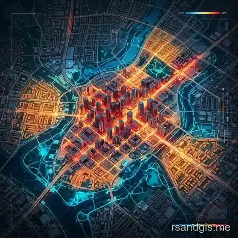
As the world experiences unprecedented rates of urbanization, natural landscapes are continually being replaced by dense concentrations of pavement, buildings, and other surfaces that absorb and retain heat. This widespread transformation of the natural environment into the built environment has given rise to one of the most critical meteorological and environmental challenges of the 21st century: the Urban Heat Island (UHI) effect. An Urban Heat Island refers to the phenomenon where urbanized areas experience significantly higher temperatures than their surrounding rural or natural peripheries. The temperature discrepancy is primarily driven by the replacement of natural vegetation, which naturally cools the environment through evapotranspiration, with impervious surfaces such as concrete and asphalt that have high thermal admittance and low albedo.

Understanding and mitigating the Urban Heat Island effect is crucial for several reasons. Elevated temperatures in urban cores lead to increased energy consumption as residents and businesses rely more heavily on air conditioning systems to maintain comfortable indoor temperatures. This, in turn, exacerbates greenhouse gas emissions, creating a vicious cycle of localized and global warming. Furthermore, the UHI effect significantly impacts public health. Heatwaves, which are amplified in urban heat islands, are among the deadliest weather-related phenomena, causing heat exhaustion, heat stroke, and exacerbating preexisting respiratory and cardiovascular conditions. Given these profound impacts, urban planners, climatologists, and environmental scientists require robust, accurate, and scalable methods to visualize, measure, and analyze heat distribution across cities. This is precisely where remote sensing technologies and Geographic Information Systems (GIS) become indispensable. In this comprehensive guide, we will delve deep into the methodologies for urban heat island mapping, leveraging the power of satellite imagery and advanced geospatial analysis.

The Role of Remote Sensing and Landsat 8

Historically, studying urban temperature variations required the deployment of dense networks of ground-based meteorological stations. While these stations provide highly accurate, continuous data for specific point locations, they are exceptionally costly to install and maintain, and they fail to capture the continuous spatial variation of temperatures across complex urban terrains. Remote sensing overcomes these limitations by providing a synoptic, bird's-eye view of the Earth's surface, capturing thermal data across vast areas simultaneously.

Among the constellation of Earth observation satellites, the Landsat program, jointly managed by NASA and the United States Geological Survey (USGS), stands out as a paramount resource. Specifically, Landsat 8, launched in February 2013, is equipped with two highly advanced sensor payloads: the Operational Land Imager (OLI) and the Thermal Infrared Sensor (TIRS). The OLI captures data across the visible, near-infrared, and shortwave-infrared spectra, which is crucial for identifying different types of land cover, such as vegetation, water bodies, and urban infrastructure. However, for the purpose of urban heat island mapping, the TIRS is the star of the show. The Landsat 8 thermal band (specifically Band 10 and Band 11) captures thermal infrared radiation emitted from the Earth's surface. Unlike visible light, which is reflected by the surface, thermal infrared radiation is a measure of the heat actually radiating from the surface itself.

The Landsat 8 thermal band data is typically provided at a spatial resolution of 100 meters, which is resampled by the USGS to 30 meters to align with the OLI optical bands. This resolution is incredibly well-suited for urban scale analysis. It is fine enough to distinguish temperature differences between a large industrial complex, a densely packed residential neighborhood, and a sprawling urban park, yet broad enough to cover an entire metropolitan region in a single satellite scene. By utilizing the Landsat 8 thermal band, researchers and GIS professionals can derive a highly detailed, spatially continuous map of surface temperatures, which forms the foundational dataset for any rigorous UHI study.

Understanding Land Surface Temperature (LST)

Before diving into the technical calculations, it is essential to distinguish between air temperature and Land Surface Temperature (LST). Air temperature, which is what we typically hear on the daily weather forecast, is the temperature of the air approximately 1.5 to 2 meters above the ground, shielded from direct solar radiation. LST, on the other hand, is how hot the surface of the Earth would feel to the touch in a particular location. It is the skin temperature of the landscape. During a sunny summer day, the LST of an asphalt parking lot can be significantly higher than the local air temperature, sometimes by tens of degrees Celsius.

For the purposes of urban heat island mapping, we focus on LST because satellite thermal sensors measure the radiant energy emitted directly from these surfaces. While LST and air temperature are related, their relationship is complex and influenced by wind, humidity, and the specific thermal properties of the surface materials. By mapping LST, we can identify the specific micro-locations—the "hot spots"—within a city that are contributing most intensely to the overall urban heat load. To accurately calculate land surface temperature from satellite imagery is a multi-step physical and mathematical process that involves converting raw digital numbers recorded by the sensor into absolute temperature values, while accounting for the atmospheric interference and the varied emissive properties of different land cover types.

The Methodology: LST Calculation Step-by-Step

The core of urban heat island mapping using Landsat 8 involves a rigorous LST calculation workflow. This process requires both the thermal bands (for temperature data) and the optical bands (for vegetation data, which is needed to calculate emissivity). The workflow generally consists of the following consecutive steps:

Step 1: Conversion to Top of Atmosphere (TOA) Spectral Radiance

When you download raw Landsat 8 data, the pixel values are represented as Digital Numbers (DN). These DNs do not represent any physical unit of measurement. The first crucial step is to convert the DNs of the thermal band (Band 10) into Top of Atmosphere (TOA) Spectral Radiance. Radiance is the amount of light (in this case, thermal energy) that reaches the satellite sensor. The conversion relies on radiance rescaling factors provided in the metadata file (MTL.txt) that accompanies the satellite imagery download. The formula is:

Lλ = ML * Qcal + AL

Where Lλ is the TOA spectral radiance, ML is the band-specific multiplicative rescaling factor, AL is the band-specific additive rescaling factor, and Qcal is the quantized and calibrated standard product pixel value (DN).

Step 2: Conversion to At-Satellite Brightness Temperature

Once you have the radiance, the next step in the LST calculation is to convert it into At-Satellite Brightness Temperature (BT). Brightness temperature is the effective temperature viewed by the satellite under the assumption that the Earth's surface acts as a black body (a perfect emitter of radiation). The calculation uses the thermal constants (K1 and K2) specific to Landsat 8 Band 10, which are also found in the metadata file. The resulting temperature is in Kelvin, which is typically converted to Celsius for easier interpretation.

BT = (K2 / ln(K1 / Lλ + 1)) - 273.15

Step 3: Calculating NDVI (Normalized Difference Vegetation Index)

Because the Earth is not a perfect black body, different surfaces emit thermal radiation with different efficiencies. This property is known as Land Surface Emissivity (LSE). To calculate LSE accurately, we need to know what type of surface we are looking at. The most common and reliable method is to use the proportion of vegetation in a pixel. To find the vegetation proportion, we first must calculate the Normalized Difference Vegetation Index (NDVI). NDVI utilizes the Near-Infrared (Band 5) and Red (Band 4) optical bands of Landsat 8. Healthy, dense vegetation reflects strongly in the near-infrared and absorbs red light, making NDVI an excellent proxy for vegetation health and density.

NDVI = (Band 5 - Band 4) / (Band 5 + Band 4)

Step 4: Calculating Proportion of Vegetation (Pv)

With the NDVI calculated, we can derive the Proportion of Vegetation (Pv), which represents the fractional area of a pixel covered by vegetation. This involves establishing the minimum NDVI value for bare soil (NDVI_min) and the maximum NDVI value for dense, healthy vegetation (NDVI_max) within the study area.

Pv = [(NDVI - NDVI_min) / (NDVI_max - NDVI_min)] ^ 2

Step 5: Calculating Land Surface Emissivity (LSE)

Emissivity is a critical factor; without it, our temperature estimates would be severely skewed. Water, vegetation, and concrete all emit heat differently. By using the Proportion of Vegetation, we can estimate the Land Surface Emissivity (LSE) for each pixel. A commonly used empirical equation estimates LSE based on Pv:

LSE = 0.004 * Pv + 0.986

Step 6: Final Land Surface Temperature (LST) Calculation

The final, culminating step to calculate land surface temperature is to correct the Brightness Temperature (BT) using the calculated Land Surface Emissivity (LSE). This correction accounts for the specific thermal emission characteristics of the landscape, providing the true Land Surface Temperature. The formula incorporates the wavelength of emitted radiance (λ = 10.8 μm for Band 10) and physical constants (Planck's constant, velocity of light, and Boltzmann constant, simplified into a single coefficient ρ = 14380).

LST = BT / [1 + (λ * BT / ρ) * ln(LSE)]

Technical Implementation: LST Calculation using Python and Rasterio

While urban heat island GIS mapping can be performed using desktop software like ArcGIS Pro or QGIS using their built-in raster calculators, utilizing Python scripting offers immense advantages in terms of automation, reproducibility, and scalability, especially when processing large time-series datasets over massive metropolitan areas. The rasterio library is a powerful and standard tool in the geospatial Python ecosystem for reading, manipulating, and writing geospatial raster data.

Below is a comprehensive Python script that automates the entire LST calculation workflow discussed above. This script reads the Landsat 8 Band 10 (thermal), Band 4 (red), and Band 5 (near-infrared) files, performs the mathematical matrix operations utilizing the highly optimized numpy library, and exports the final Land Surface Temperature map as a new GeoTIFF file ready for further urban heat island gis analysis.

import rasterio
import numpy as np
import warnings

# Suppress warnings for invalid values in calculations (e.g., division by zero, log of negative numbers)
warnings.filterwarnings('ignore')

def calculate_lst(b10_path, b4_path, b5_path, output_path):
    print("Starting LST Calculation...")
    
    # ---------------------------------------------------------
    # 1. Define Landsat 8 Constants from Metadata (MTL file)
    # ---------------------------------------------------------
    # Note: These values are standard for Landsat 8, but always verify with your specific scene's MTL file.
    M_L = 0.0003342    # RADIANCE_MULT_BAND_10
    A_L = 0.1          # RADIANCE_ADD_BAND_10
    K1 = 774.8853      # K1_CONSTANT_BAND_10
    K2 = 1321.0789     # K2_CONSTANT_BAND_10
    wavelength = 10.8  # Wavelength of Band 10 in micrometers
    p = 14380.0        # p = h * c / s (Planck's constant * velocity of light / Boltzmann constant)

    # ---------------------------------------------------------
    # 2. Read Raster Data using Rasterio
    # ---------------------------------------------------------
    print("Loading raster bands...")
    with rasterio.open(b10_path) as src_b10:
        band10 = src_b10.read(1).astype(np.float32)
        meta = src_b10.meta # Copy spatial metadata for the output file
        # Mask out NoData values (typically 0 in Landsat)
        nodata = src_b10.nodata if src_b10.nodata is not None else 0
        mask = (band10 == nodata)

    with rasterio.open(b4_path) as src_b4:
        band4 = src_b4.read(1).astype(np.float32)

    with rasterio.open(b5_path) as src_b5:
        band5 = src_b5.read(1).astype(np.float32)

    # ---------------------------------------------------------
    # 3. Perform Calculations
    # ---------------------------------------------------------
    
    # Step 1: TOA Radiance
    print("Calculating TOA Radiance...")
    L_lambda = (M_L * band10) + A_L
    L_lambda[L_lambda <= 0] = np.nan # Prevent log of zero or negative later

    # Step 2: At-Satellite Brightness Temperature (Celsius)
    print("Calculating Brightness Temperature...")
    BT = (K2 / (np.log((K1 / L_lambda) + 1.0))) - 273.15

    # Step 3: NDVI Calculation
    print("Calculating NDVI...")
    denominator = (band5 + band4)
    # Avoid division by zero
    denominator[denominator == 0] = np.nan
    ndvi = (band5 - band4) / denominator

    # Step 4: Proportion of Vegetation (Pv)
    print("Calculating Proportion of Vegetation...")
    # Dynamically find the min and max NDVI values, ignoring NaNs
    ndvi_min = np.nanmin(ndvi)
    ndvi_max = np.nanmax(ndvi)
    
    # Clip NDVI to strictly remain within min/max bounds to avoid anomalous Pv values
    ndvi_clipped = np.clip(ndvi, ndvi_min, ndvi_max)
    pv = ((ndvi_clipped - ndvi_min) / (ndvi_max - ndvi_min)) ** 2

    # Step 5: Land Surface Emissivity (LSE)
    print("Calculating Land Surface Emissivity...")
    lse = 0.004 * pv + 0.986
    lse[lse <= 0] = np.nan

    # Step 6: Final Land Surface Temperature (LST)
    print("Calculating final Land Surface Temperature...")
    lst = BT / (1.0 + (wavelength * BT / p) * np.log(lse))

    # Re-apply the mask to remove data outside the satellite footprint
    lst[mask] = np.nan

    # ---------------------------------------------------------
    # 4. Export the Result
    # ---------------------------------------------------------
    print(f"Exporting final LST map to {output_path}...")
    meta.update(
        dtype=rasterio.float32,
        count=1,
        nodata=np.nan,
        compress='lzw' # Add compression to save disk space
    )
    
    with rasterio.open(output_path, 'w', **meta) as dst:
        dst.write(lst, 1)
        
    print("LST Calculation Complete!")

# Example usage (Ensure you replace these paths with your actual file paths)
# calculate_lst('LC08_L1TP_B10.TIF', 'LC08_L1TP_B4.TIF', 'LC08_L1TP_B5.TIF', 'UHI_LST_Output.tif')

Exploring the NDVI and LST Relationship

Once the Land Surface Temperature raster is generated, the next vital phase in urban heat island mapping is rigorous spatial and statistical analysis. One of the most fundamental and widely researched aspects of UHI studies is the inverse correlation inherent in the NDVI and LST relationship. Extensive global research consistently demonstrates a strong negative correlation between the Normalized Difference Vegetation Index (NDVI) and Land Surface Temperature (LST) within urban environments. As NDVI values increase—indicating denser, healthier vegetation canopies—LST values reliably decrease. This is not a mere coincidence; it is driven by complex biophysical processes.

Urban vegetation, such as street trees, parks, and green roofs, provides profound cooling effects through two primary mechanisms: shading and evapotranspiration. Shading physically blocks shortwave solar radiation from striking and heating impervious surfaces like asphalt and concrete. Evapotranspiration is the biological process by which plants absorb water through their roots and release it as water vapor through their stomata. This phase change of water from liquid to gas absorbs a significant amount of latent heat from the surrounding environment, thereby actively cooling the ambient air and the surface. By overlaying the NDVI raster map with the calculated LST raster in a GIS environment, urban planners can quantitatively prove the efficacy of urban greening initiatives. Analyzing the NDVI and LST relationship allows city administrators to strategically target barren, highly impervious zones with new green infrastructure projects, maximizing the cooling return on investment.

Advanced Urban Heat Island GIS Techniques

Creating the LST map is merely the foundation of urban heat island gis applications. To derive actionable insights that can influence public policy and urban design, advanced GIS techniques must be applied to the LST dataset.

• Zonal Statistics and Land Use Analysis: By overlaying the continuous LST raster with discrete vector polygon layers representing urban land use categories (e.g., residential, commercial, industrial, parks), analysts can utilize Zonal Statistics to calculate the mean, maximum, and minimum temperatures for each specific land use type. This analysis often reveals that sprawling industrial zones and massive commercial parking lots are the most severe contributors to the UHI effect, while mature residential neighborhoods with significant tree canopy cover remain substantially cooler.
• Hotspot Analysis (Getis-Ord Gi*): Rather than just looking at raw temperature values, spatial statistics tools like Getis-Ord Gi* can be employed to identify statistically significant spatial clusters of high values (hot spots) and low values (cold spots). This helps differentiate areas that are genuinely anomalous from those experiencing normal temperature fluctuations, providing urban planners with empirically validated target zones for heat mitigation strategies, such as implementing cool roof incentive programs or targeted urban afforestation.
• Vulnerability Mapping: The true power of urban heat island gis is realized when environmental data is intersected with socioeconomic demographic data. By combining the UHI hot spot maps with census data representing vulnerable populations—such as the elderly, young children, low-income households, and communities lacking access to central air conditioning—GIS analysts can create comprehensive Heat Vulnerability Indices. These maps are critical for emergency management agencies to deploy cooling centers, direct outreach programs, and allocate resources efficiently during extreme, life-threatening heatwave events.

Conclusion

Mapping Urban Heat Islands is no longer an esoteric academic exercise; it is an absolute necessity for sustainable, resilient urban planning in the face of accelerating global climate change. Through the powerful synergy of the Landsat 8 thermal band and advanced Geographic Information Systems, researchers and city managers possess the exact tools required to visualize, quantify, and analyze the complex spatial dynamics of urban heat. By meticulously executing the LST calculation workflow—converting digital numbers to radiance, extracting brightness temperature, and utilizing the NDVI and LST relationship to determine emissivity—we can produce highly accurate, high-resolution thermal maps. Whether utilizing desktop GIS software or powerful Python libraries like rasterio for automated, large-scale analysis, the insights derived from urban heat island mapping are crucial for designing cooler, healthier, and more equitable cities for the future.