automated landslide detection using sentinel-2 and python

AI & ML August 18, 2026

The growing frequency and severity of natural disasters across the globe necessitate the development of robust, scalable, and responsive monitoring systems. Among the most destructive of these natural hazards are landslides, which can cause immense damage to infrastructure, alter landscapes permanently, and result in significant loss of life. In this comprehensive, technical guide, we will thoroughly explore automated landslide detection using sentinel-2 and python. By leveraging the power of modern satellite imagery—specifically the high-resolution optical data provided by the European Space Agency's Copernicus program—developers, researchers, and geographic information system (GIS) professionals can identify critical environmental changes in near real-time. Throughout this meticulously detailed article, we will delve deeply into the theoretical underpinnings of vegetation indices, the practical applications of NDVI differencing, image thresholding techniques, and the construction of complete Python-based workflows designed to entirely automate the mapping and analytical process from start to finish.

1. Introduction to Remote Sensing for Disaster Management

Remote sensing has fundamentally transformed the way humanity interacts with and understands the Earth's surface. In the context of disaster management and emergency response, satellite imagery offers an unparalleled vantage point. Historically, mapping landslides required extensive, dangerous, and time-consuming field surveys, supplemented by expensive aerial photography flown from planes or helicopters. This traditional approach meant that hazard maps were often severely outdated by the time they were published, offering little immediate help to crisis responders dealing with fresh, ongoing emergencies.

Today, a massive constellation of Earth observation satellites continuously orbits the planet, passively collecting petabytes of multispectral data every single day. This continuous stream of data allows scientists to perform rapid temporal analyses, comparing the state of the environment immediately before and after a triggering event, such as a major earthquake, a typhoon, or a prolonged period of extreme rainfall. When a landslide occurs, it typically strips away the overlying vegetation and exposes bare soil, bedrock, and debris. This dramatic physical alteration of the landscape produces a distinctly measurable change in how the surface reflects electromagnetic radiation, particularly in the visible and near-infrared portions of the spectrum. By detecting these spectral changes algorithmically, we can map thousands of landslides across vast, inaccessible mountainous regions in a matter of hours—a task that would otherwise take human surveyors years to complete manually. Python, with its rich, ever-expanding ecosystem of data science and geospatial libraries, serves as the perfect programmable glue to tie these advanced remote sensing concepts into a cohesive, highly automated processing pipeline.

2. The Sentinel-2 Mission: Optical Earth Observation

The Sentinel-2 mission, developed, launched, and operated by the European Space Agency (ESA) as a cornerstone of the broader European Union Copernicus program, consists of twin satellites: Sentinel-2A and Sentinel-2B. These two identical satellites are phased at exactly 180 degrees to each other on the same sun-synchronous orbit, providing an exceptional revisit time of just five days at the equator, and even more frequently at mid-latitudes (often every 2-3 days). This incredibly high temporal resolution is critical for effective disaster monitoring, as it dramatically maximizes the statistical probability of obtaining completely cloud-free imagery immediately following a sudden disaster event.

What truly sets Sentinel-2 apart from historical missions like Landsat, however, is its advanced Multispectral Instrument (MSI). The MSI captures data across 13 distinct spectral bands, spanning the visible, near-infrared (NIR), and shortwave infrared (SWIR) wavelengths. Crucially for our purposes, the primary visible bands (Red, Green, Blue) and the broad Near-Infrared band (Band 8) are captured at an unprecedented spatial resolution of 10 meters per pixel. This 10-meter resolution provides a beautiful, highly effective balance between broad, regional spatial coverage and the granular, fine-scale detail necessary to detect medium to large-scale mass movements. Additionally, Sentinel-2 includes specialized "red edge" bands designed specifically for monitoring subtle changes in vegetation health, though these are captured at a slightly coarser 20-meter resolution. The fact that this incredible, research-grade dataset is freely and openly available to the global public has democratized Earth observation. It allows individual researchers, university students, and small non-governmental organizations (NGOs) to build sophisticated, automated monitoring tools without incurring the traditionally prohibitive data acquisition costs associated with commercial satellite operators.

3. The Mechanics of Landslides and Their Spectral Signatures

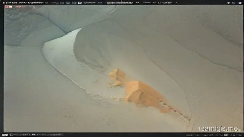
To accurately detect a landslide using optical remote sensing, one must first fundamentally understand what a landslide physically does to the terrain it occupies. A landslide is broadly defined in geology as the movement of a mass of rock, debris, or earth down a slope under the direct influence of gravity. This movement is typically triggered by external forcing factors such as heavy, sustained precipitation, violent seismic activity, volcanic eruptions, or direct human interference such as extensive deforestation, mining, and road construction on unstable slopes. When the massive volume of earth moves, it invariably destroys and carries away the existing land cover.

In heavily forested or vegetated regions—where landslides are often most prevalent due to steep terrain and loose, waterlogged soils—the sudden removal of trees, shrubs, and deep-rooted grasses is the primary, most obvious signal we look for from space. Healthy, photosynthesizing vegetation strongly absorbs visible red light (used as fuel for photosynthesis) while simultaneously strongly reflecting near-infrared light due to the complex internal spongy mesophyll cellular structure of the leaves. When a landslide suddenly strips the vegetation away and exposes the underlying mineral soil or bedrock, this established spectral signature flips dramatically. Bare soil reflects much more red light than a dense forest canopy and reflects significantly less near-infrared light. This distinct, immediate spectral contrast between "pre-event vegetated" and "post-event bare" surfaces forms the absolute theoretical foundation of our automated detection methodology. By mathematically isolating this specific change in the spectral signature, we can reliably separate new landslides from other, slower land cover changes, such as seasonal vegetation phenology (the natural browning of leaves in autumn) or gradual urban development.

4. Normalized Difference Vegetation Index (NDVI) Explained

The Normalized Difference Vegetation Index (NDVI) is arguably the most famous, widely utilized, and universally understood spectral index in the entire field of remote sensing. It is a dimensionless metric that quantifies the density, greenness, and overall health of vegetation in a given pixel. The formula for calculating NDVI relies entirely on the inverse relationship between the near-infrared (NIR) and visible red (RED) bands that we discussed in the previous section. For Sentinel-2 data, this specifically corresponds to Band 8 (the broad Near-Infrared band) and Band 4 (the visible Red band).

The globally accepted mathematical formula is expressed simply as: NDVI = (NIR - RED) / (NIR + RED)

Because it is a normalized ratio, calculated by dividing the difference by the sum, NDVI values inherently fall strictly between the boundaries of -1.0 and +1.0. High positive values (for example, ranging from 0.6 to 0.9) indicate dense, highly active, and healthy green vegetation, such as a thriving tropical rainforest canopy or a mature agricultural crop. Values closer to zero (for example, 0.0 to 0.2) typically represent non-vegetated surfaces like bare soil, exposed rock outcroppings, or dense urban infrastructure. Negative values are generally associated with water bodies, deep snow, ice, or thick, opaque clouds, as these physical features actually reflect more visible red light than near-infrared light. By computing the NDVI for an entire satellite image, we effectively transform a complex, multi-dimensional multispectral dataset into a heavily simplified, single-band grayscale map of vegetation density. This transformation is highly computationally efficient, making it absolutely ideal for inclusion in an automated processing pipeline where execution speed, memory management, and scalability are primary considerations for developers.

5. NDVI Differencing (dNDVI) for Change Detection

While calculating a single NDVI image can tell us exactly where vegetation is currently located at one specific moment in time, it cannot inherently tell us where a landslide has recently occurred. To achieve actual detection, we must employ a temporal change detection technique formally known as NDVI differencing (often abbreviated as dNDVI or delta-NDVI). This process involves acquiring two completely cloud-free satellite images over the exact same geographic bounding box: one image captured immediately before the disaster event (referred to in the literature as T0, or the pre-event image) and one image captured immediately after the event has concluded (referred to as T1, or the post-event image).

First, we calculate the standard NDVI for both the pre-event and post-event images entirely independently. Let's designate these two resulting arrays as NDVI_pre and NDVI_post. We then perform a simple mathematical subtraction: we subtract the post-event NDVI from the pre-event NDVI to calculate the absolute difference (dNDVI).

The core formula is simply: dNDVI = NDVI_pre - NDVI_post

Let us carefully trace the logical flow of this subtraction operation. Before a massive landslide occurs, a densely forested mountain slope will possess a very high NDVI value (e.g., 0.85). After the landslide completely destroys the forest and exposes bare, un-vegetated soil, the NDVI of that exact same pixel location will drop significantly (e.g., plunging to 0.15). Subtracting the post-event value from the pre-event value yields a large, positive difference (0.85 - 0.15 = 0.70). Conversely, surrounding areas of the forest that remained completely undisturbed will possess very similar pre- and post-event NDVI values, resulting in a dNDVI value that hovers very close to zero. Therefore, pixels exhibiting a highly positive dNDVI represent distinct areas where vegetation was suddenly, violently, and drastically removed—which is the exact spectral fingerprint of a recent landslide. This simple, elegant, yet profoundly powerful mathematical operation is the true engine that drives our automated processing logic.

6. Determining the Right Thresholds for Classification

Once we have successfully computed our continuous dNDVI raster surface, we must convert this gradient of values into a strict, binary classification map: a pixel is either a landslide, or it is not a landslide. This critical conversion is achieved through a technique known as image thresholding. A threshold is a specific, carefully chosen numerical value used to partition our continuous data into discrete classes. If a given pixel's dNDVI value is strictly greater than the chosen threshold, we confidently classify it as a landslide; if it is less than or equal to the threshold, we classify it as stable background or an unrelated, benign environmental change.

Selecting the mathematically correct threshold is often considered the most challenging, nuanced, and error-prone aspect of this entire automated workflow. If the threshold is set too low (e.g., 0.1), the algorithm will be overly sensitive and incredibly "noisy." It will successfully capture all the real landslides, but it will simultaneously flag thousands of false positives caused by subtle, natural seasonal changes in leaf coloration, slight atmospheric discrepancies between the two orbital passes, or minor, localized agricultural harvesting. Conversely, if the threshold is set too high (e.g., 0.7), the algorithm will be excessively conservative, entirely missing shallow, smaller landslides or areas where the original vegetation was only partially damaged rather than completely obliterated. Often, a static threshold value somewhere between 0.3 and 0.5 is empirically found to be optimal for identifying major mass wasting events in heavily forested, mountainous regions. In a truly automated, production-grade enterprise system, this threshold might not be rigidly hardcoded at all. Instead, it could be dynamically calculated on the fly using advanced statistical methods like Otsu's binarization, or by carefully evaluating the standard deviation of the dNDVI histogram exclusively across an area known to be geologically stable.

7. Python Environment Setup: The Geospatial Stack

Python has rapidly ascended to become the undisputed lingua franca of modern geospatial data science and Earth observation analytics. To properly implement our automated landslide detection workflow, we need to construct a highly robust, dedicated Python environment equipped with exactly the right specialized libraries. We will completely bypass heavy, proprietary, point-and-click desktop GIS software (which is difficult to automate) in favor of lightweight, open-source Python packages that can be executed rapidly and headlessly on remote servers, Docker containers, or distributed cloud computing infrastructure.

The core suite of Python libraries we absolutely require includes:

• Rasterio: This fantastic library is the modern, accepted standard for reading, writing, and manipulating geospatial raster data in Python. It provides a highly Pythonic, intuitive interface to the powerful but complex underlying C-based GDAL library, allowing us to read massive Sentinel-2 GeoTIFF files directly into computer memory as multi-dimensional NumPy arrays effortlessly.
• NumPy: The foundational, fundamental package for all scientific computing in Python. We will rely heavily on NumPy to perform the incredibly fast, vectorized array mathematics required to calculate NDVI and dNDVI equations across tens of millions of pixels simultaneously, without relying on slow Python "for" loops.
• Geopandas: A brilliant extension of the wildly popular Pandas library, specifically designed to handle vector geometries (points, lines, and complex polygons). Once we successfully detect landslide pixels in our raster imagery, we will convert these distinct pixel clusters into smooth vector polygons using Geopandas for easy database storage, spatial querying, and web-map visualization.
• SciPy: Specifically, we will utilize the scipy.ndimage module, which provides essential, highly optimized tools for multi-dimensional morphological image processing. We will use this module to meticulously clean up our binary classification mask, programmatically removing tiny, isolated pixels of statistical noise that do not realistically represent genuine landslides.

Setting up this complex environment is most safely and typically done using the Conda package manager (or Miniforge). Conda expertly and seamlessly handles the notoriously complex underlying C/C++ library dependencies (like PROJ and GEOS) that geospatial tools invariably require to function correctly. Creating an entirely isolated, dedicated Conda environment ensures that our workflow remains highly reproducible, completely stable, and easily transferable across different operating systems and developer machines.

8. Data Acquisition and Preprocessing Best Practices

Before any developer can write a single line of analytical processing code, one must first successfully acquire the raw satellite data. For fully automated, production-ready systems, relying on humans to manually browse and download files from web portals is completely insufficient and unscalable. Instead, developers should heavily utilize robust REST APIs provided by modern geospatial platforms like the Copernicus Data Space Ecosystem, Microsoft's Planetary Computer, or the Google Earth Engine Python API. These platforms allow our Python scripts to programmatically search massive catalogs for Sentinel-2 imagery that strictly intersects a specific geographic bounding box, exclusively within a tightly defined chronological time window immediately spanning the disaster.

Once the correct imagery scenes are identified and downloaded, rigorous preprocessing is absolutely vital to the success of the algorithm. The single biggest enemy of optical remote sensing is, without a doubt, cloud cover. Because the Sentinel-2 MSI instrument cannot physically see through atmospheric clouds, any cloud or dark cloud shadow appearing in either the pre-event or post-event image will completely ruin the NDVI calculation for those specific pixels, inevitably leading to massive clusters of glaring false positives. Therefore, the very first, non-negotiable step in our processing pipeline is applying a robust, mathematically rigorous cloud mask. Fortunately, official Sentinel-2 Level-2A data products come conveniently packaged with a dedicated Scene Classification Layer (SCL) that intelligently identifies clouds, cloud shadows, snow, and surface water. We must write custom Python code to read this specific SCL band and deliberately mask out (set to NaN) any non-clear pixels in our corresponding Red and NIR arrays.

Furthermore, atmospheric correction is not just recommended; it is strictly necessary. We must meticulously ensure we are exclusively using Level-2A data (representing Bottom of Atmosphere reflectance) rather than raw Level-1C data (representing Top of Atmosphere reflectance). Level-2A data has been mathematically corrected for complex atmospheric scattering, aerosol interference, and water vapor absorption, ensuring that the spectral values we analyze truly, accurately represent the physical surface of the Earth. This crucial correction makes our direct NDVI comparisons across time mathematically valid, physically meaningful, and highly defensible.

9. Step-by-Step Implementation: Calculating NDVI with Python

Let's dive directly into the core Python implementation of the theory we have discussed. Assuming we have successfully downloaded our pre-event and post-event Sentinel-2 Level-2A scenes, securely applied our cloud masks, and extracted the 10-meter Red (Band 4) and NIR (Band 8) GeoTIFF files to our local disk, we begin by reading them directly into active memory using the Rasterio library. Note carefully that we will explicitly configure NumPy to suppress and ignore "divide-by-zero" warnings, which can occasionally occur if a pixel happens to possess a highly unusual value of exactly zero in both the Red and NIR bands simultaneously.

import rasterio
import numpy as np

def calculate_ndvi_safely(red_file_path, nir_file_path):
    # Open the raster datasets using context managers to ensure they close properly
    with rasterio.open(red_file_path) as red_dataset, rasterio.open(nir_file_path) as nir_dataset:
        # Read the first band of each dataset into a NumPy array, cast to float for division
        red_band = red_dataset.read(1).astype(float)
        nir_band = nir_dataset.read(1).astype(float)
        
        # Configure NumPy to quietly ignore division by zero or invalid floating point operations
        np.seterr(divide='ignore', invalid='ignore')
        
        # Execute the core NDVI formula using fast vectorized operations
        calculated_ndvi = (nir_band - red_band) / (nir_band + red_band)
        
        # Safely handle any NaN (Not a Number) values resulting from division by zero
        # We replace them with -1.0, which clearly indicates non-vegetation
        calculated_ndvi = np.nan_to_num(calculated_ndvi, nan=-1.0)
        
        # Return both the calculated array and the spatial profile metadata for later use
        return calculated_ndvi, red_dataset.profile

# Execute the function for both the T0 (pre-event) and T1 (post-event) timeframes
ndvi_pre_event, spatial_profile = calculate_ndvi_safely('T0_B04.tif', 'T0_B08.tif')
ndvi_post_event, _ = calculate_ndvi_safely('T1_B04.tif', 'T1_B08.tif')

This well-structured code snippet forms the absolute bedrock of our entire automated analysis. By abstracting the complex file reading and mathematical calculation into a dedicated, reusable, and cleanly defined Python function, our overarching automated workflow remains beautifully clean, modular, and easy to test. The resulting ndvi_pre_event and ndvi_post_event variables stored in memory are now massive, two-dimensional NumPy arrays, with floating-point values ranging continuously and strictly from -1.0 to 1.0, mathematically representing the precise state of the vegetation canopy immediately before and immediately after the triggering disaster event.

10. Step-by-Step Implementation: Differencing and Thresholding

With our pre and post NDVI arrays successfully computed and residing in memory, the next highly logical step in the automated pipeline is to calculate the absolute temporal difference and forcefully apply our carefully selected, geologically appropriate threshold. This specific block of code is exactly where the actual "detection" magically takes place. Because the NumPy library is incredibly highly optimized for running vectorized mathematical operations in compiled C code beneath the surface, this massive calculation happens almost instantaneously—even for full Sentinel-2 spatial tiles containing well over 100 million individual pixels.

# Calculate the critical temporal difference in NDVI
# Positive values indicate a loss of vegetation; negative values indicate growth
dndvi_array = ndvi_pre_event - ndvi_post_event

# Define our highly specific, empirically tested detection threshold
# In this scenario, a drop of 0.35 in NDVI is required to flag a pixel
detection_threshold = 0.35

# Create a strict binary classification mask using a boolean condition
# We cast the resulting boolean array (True/False) to unsigned 8-bit integers (1/0)
# 1 = Potential Landslide Pixel, 0 = Stable Background Pixel
raw_landslide_mask = (dndvi_array > detection_threshold).astype(np.uint8)

In this concise but incredibly powerful block of code, we methodically subtract the post-event array directly from the pre-event array. We then establish our strict operating threshold of 0.35. Any individual pixel where the calculated vegetation index dropped by a margin strictly greater than 0.35 between the two satellite overpasses is instantly flagged as a True (represented as a 1) in our resulting boolean mask, while everything else gracefully becomes False (represented as a 0). This binary raw_landslide_mask is our raw, highly unrefined map of potential landslides. However, as with absolutely any automated remote sensing technique running on real-world data, this raw output will inevitably contain significant amounts of noise that absolutely must be addressed before the data can be considered safe or useful for actual disaster responders or civil engineers.

11. Post-Processing: Filtering Noise and Exporting to Vector

The raw, freshly generated binary mask will undoubtedly contain numerous "salt and pepper" false positives—tiny, isolated clusters of one, two, or three pixels that artificially triggered the threshold due to random sensor noise, minor sub-pixel co-registration errors between the two satellite orbital passes, or a single, highly localized fallen tree. A real, dangerous landslide is generally much, much larger than a mere 10 or 20 square meters. To effectively and programmatically remove this distracting noise, we apply mathematical morphological operations from the SciPy library, specifically utilizing a binary opening operation or an area-based sieve. After thoroughly cleaning the raster array, we use the Rasterio features module to seamlessly convert the distinct, validated clumps of pixels into smooth vector polygons, which we then easily save as a standard shapefile or GeoJSON format utilizing the Geopandas library.

import geopandas as gpd
from rasterio.features import shapes
from scipy.ndimage import binary_opening, generate_binary_structure

# Define a strict 3x3 structural element matrix for the morphological opening operation
# This defines what constitutes a "connected" group of pixels
morph_structure = generate_binary_structure(2, 2)

# Execute the opening operation to strip away tiny, isolated noise pixels
# This preserves large, continuous blobs (real landslides) while deleting single pixels
cleaned_mask = binary_opening(raw_landslide_mask, structure=morph_structure).astype(np.uint8)

# Programmatically convert the cleaned raster mask into geometric vector polygons
polygon_results = []
# Iterate through all generated shapes, applying the spatial transform for coordinates
for geometric_shape, pixel_value in shapes(cleaned_mask, transform=spatial_profile['transform']):
    if pixel_value == 1:  # We are only interested in keeping the actual landslide polygons
        polygon_results.append({
            'geometry': geometric_shape, 
            'properties': {'classification': 'landslide_event'}
        })

# Create a powerful Geopandas GeoDataFrame from the resulting dictionary list
final_gdf = gpd.GeoDataFrame.from_features(polygon_results, crs=spatial_profile['crs'])

# Export the final, cleaned vector dataset to a highly portable GeoJSON file
final_gdf.to_file('automatically_detected_landslides.geojson', driver='GeoJSON')

This final, crucial step successfully bridges the highly technical gap between grid-based raster analysis and traditional, feature-based GIS mapping. By outputting standard, universally accepted vector formats like GeoJSON, our highly automated Python script rapidly produces lightweight data that can immediately, seamlessly be ingested into interactive web mapping applications, real-time disaster dashboards, or heavy desktop software like QGIS and Esri ArcGIS for final human validation and widespread dissemination to critical emergency management agencies.

12. Future Directions: Topographic Data & Machine Learning

While the highly optimized NDVI differencing and thresholding approach detailed extensively in this guide is incredibly powerful, accessible, and highly computationally efficient, it is certainly not without its inherent scientific limitations. Its absolute primary weakness is that it technically detects *all* sudden, drastic vegetation loss, not just actual geological landslides. A completely unrelated fresh clear-cut logging operation, a rapidly spreading natural wildfire, or massive new road construction will also produce extremely high dNDVI values and be falsely, aggressively flagged as a landslide by a purely, blindly spectral algorithm.

To intelligently mitigate this major issue in advanced, enterprise-grade automated systems, we must strategically incorporate additional, highly contextual datasets, most notably high-resolution topography. Landslides, by their very physical definition, occur exclusively on slopes. By formally introducing a Digital Elevation Model (DEM)—such as the excellent, globally available Copernicus 30m DEM or the SRTM dataset—we can programmatically calculate the exact slope angle for every single pixel in our study area. We can then confidently apply a secondary, topographic threshold, ruthlessly masking out any "detected" landslide that occurs on terrain flatter than, for example, 10 or 15 degrees, thereby instantly and elegantly eliminating massive swaths of false positives caused by agriculture, logging, or urban expansion situated perfectly in flat river valleys.

Furthermore, the cutting-edge future of automated landslide detection using sentinel-2 and python is rapidly and decisively shifting towards the incredibly exciting fields of Machine Learning (ML) and Deep Learning. Instead of relying entirely on rigid, hardcoded, human-defined thresholds, modern computer vision pipelines are actively beginning to utilize highly complex Convolutional Neural Networks (CNNs) like the U-Net architecture. By exhaustively training these massive neural networks on thousands upon thousands of manually labeled, historically validated landslide examples alongside multi-temporal Sentinel-2 data and complex topographic variables, the algorithms rapidly learn to organically recognize the complex spatial textures, dendritic shapes, and subtle contextual clues of true landslides, far exceeding the raw accuracy of simple spectral differencing alone. However, the foundational thresholding method painstakingly described in this article remains the absolute, non-negotiable bedrock upon which all these advanced ML models are initially built, providing the strictly necessary baseline scientific understanding of exactly how land cover changes fundamentally manifest in optical satellite imagery.

13. Case Studies and Real-World Applications

The technical methodologies heavily discussed and outlined in this comprehensive guide are not merely academic, theoretical exercises destined to remain in textbooks; they are actively, aggressively deployed in massive real-world scenarios right now by international space agencies, elite academic institutions, and frontline disaster response organizations globally. For instance, immediately following the utterly devastating 2015 Gorkha earthquake in Nepal, pioneering researchers utilized highly similar semi-automated spectral differencing techniques on rapid-response satellite imagery to accurately map tens of thousands of violent co-seismic landslides across the inaccessible high Himalayas. This critically important, time-sensitive spatial data was delivered directly and rapidly to frantic humanitarian organizations operating on the ground, helping them efficiently identify totally blocked mountain passes and aggressively prioritize remote villages that were completely cut off from all traditional avenues of emergency aid.

Even more recently, fully automated, continuous pipelines running headlessly on massive cloud computing platforms like Google Earth Engine or Amazon Web Services (AWS) are being heavily configured to run 24 hours a day, 7 days a week. These impressive "always-on" sentinel systems constantly monitor highly geologically susceptible regions—such as the steep Andes in South America, the densely populated mountainous provinces of Southeast Asia, and the rugged Pacific Northwest of the United States—instantly triggering automated alerts to authorities whenever significant, anomalous NDVI drops strongly coincide with documented heavy rainfall events. By maintaining a constant, utterly untiring, automated digital vigil from space, these systems boldly provide early, actionable warnings that can literally and frequently mean the absolute difference between life and death for incredibly vulnerable communities residing directly downstream from highly unstable, threatening slopes. The ongoing, successful transition from slow, reactive manual mapping to rapid, proactive, continuous automated monitoring represents the true, undeniable triumph of deeply integrating Python scripting architectures with freely available Copernicus optical data.

14. Conclusion

The profound technical ability to rapidly, accurately, and continuously monitor the Earth's fragile surface for catastrophic, sudden changes is undoubtedly one of the most vital, life-saving applications of modern satellite technology in the 21st century. Developing and maintaining a highly optimized workflow for automated landslide detection using sentinel-2 and python boldly empowers dedicated researchers and frontline emergency responders to meticulously map massive disaster zones at a spatial scale and processing speed that was previously considered completely unimaginable just a decade ago. By intelligently combining the unprecedented high temporal and spatial resolution of the European Sentinel-2 constellation with the immense, highly scalable data processing capabilities of modern open-source Python libraries like Rasterio, NumPy, and Geopandas, we can effectively create scalable, robust pipelines that rapidly transform raw, unstructured pixels into highly actionable, life-saving geographical intelligence. While complex technical challenges such as pervasive cloud cover and inevitable spectral confusion certainly remain, the careful, deliberate integration of rigorous NDVI differencing, mathematical morphological post-processing, and strict topographic constraints provides a highly robust, scientifically validated, and endlessly repeatable methodology. As ongoing global climate change unfortunately continues to drastically alter historical weather patterns and drastically increase the frequency of extreme precipitation events globally, these incredibly powerful, automated Python-driven tools will only become exponentially more critical in our collective, global efforts to properly understand, aggressively mitigate, and rapidly respond to the devastating, tragic impacts of landslides worldwide.