Spatial Econometrics Models In Python
Table of Contents
- Introduction to Spatial Econometrics
- The Importance of Spatial Data
- Limitations of Traditional Econometrics
- Understanding Spatial Econometrics Models in Python
- Why Choose Python?
- Essential Libraries: PySAL, GeoPandas, and More
- Core Concepts in Spatial Econometrics
- Spatial Autocorrelation
- Spatial Weights Matrices (W)
- Types of Spatial Econometrics Models
- The Spatial Autoregressive Model (SAR)
- The Spatial Error Model (SEM)
- The Spatial Durbin Model (SDM)
- The General Spatial Model (SAC/SARMA)
- Setting Up Your Python Environment
- Installation and Dependencies
- Data Preparation with GeoPandas
- Implementing Spatial Econometrics Models in Python
- Step 1: Loading and Inspecting the Data
- Step 2: Creating the Spatial Weights Matrix
- Step 3: Testing for Spatial Autocorrelation
- Step 4: Fitting the Spatial Lag Model (SAR)
- Step 5: Fitting the Spatial Error Model (SEM)
- Step 6: Fitting the Spatial Durbin Model (SDM)
- Interpreting Spatial Econometrics Models
- Direct and Indirect Effects (Spillovers)
- Evaluating Model Fit and Diagnostics
- Advanced Topics and Best Practices
- Dealing with Missing Data and Heteroskedasticity
- Choosing the Right Spatial Weights Matrix
- Scaling to Large Spatial Datasets
- Conclusion
- Frequently Asked Questions
rsandgis.me
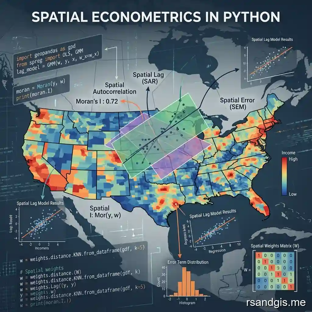
In the modern era of data science, geography and location have become pivotal in understanding economic and social phenomena. Traditional linear regression models often fall short when dealing with data that inherently possesses spatial dependencies. If you are looking to master the implementation of spatial econometrics models in python, you are in the right place. By explicitly incorporating spatial relationships into statistical analyses, researchers can uncover deeper insights. This guide will provide a detailed exploration of how to build, evaluate, and interpret these sophisticated models using powerful libraries like PySAL, GeoPandas, and statsmodels.
Introduction to Spatial Econometrics
Spatial econometrics is a specialized subfield of econometrics that specifically deals with the incorporation of spatial interaction and spatial structure into regression analysis. While traditional econometrics heavily relies on the assumption that observations are strictly independent of one another, spatial econometrics recognizes a fundamental geographic truth: "everything is related to everything else, but near things are more related than distant things." This concept, famously known as Tobler's First Law of Geography, forms the theoretical foundation for incorporating spatial weights into statistical models. This principle is absolutely fundamental when analyzing data collected across different geographic locations, such as individual census tracts, municipalities, counties, states, or even sovereign countries.
The primary reason for developing and utilizing specialized models for spatial data is the widespread presence of spatial dependence and spatial heterogeneity. Spatial dependence, frequently referred to as spatial autocorrelation, occurs when the observed value of a specific variable at one geographic location is systematically correlated with the value of the exact same variable at geographically neighboring locations.
For example, consider real estate markets: housing prices in a specific residential neighborhood are highly likely to be very similar to housing prices in immediately adjacent neighborhoods due to shared local amenities, school district quality, crime rates, and broad socioeconomic factors. If this inherent spatial dependence is ignored in a standard ordinary least squares (OLS) regression analysis, the resulting parameter estimates can be biased, inconsistent, or highly inefficient, invariably leading to incorrect inferences and potentially disastrous policy recommendations.
Spatial heterogeneity, on the other hand, refers to the structural instability of relationships across geographic space. The fundamental relationship between individual income levels and educational attainment, for instance, might be structurally and fundamentally different in densely populated urban metropolitan areas compared to sparsely populated rural agricultural areas. Spatial econometrics provides the rigorous methodological framework required to explicitly model and quantify these complex spatial effects, allowing analysts to obtain much more robust and statistically reliable empirical results. As spatial data becomes increasingly abundant and widely accessible through open data initiatives, the demand for sophisticated spatial analysis techniques has surged exponentially across various academic disciplines and industry sectors, including regional science, urban economics, environmental studies, epidemiology, and public health.
The Importance of Spatial Data
In today's highly data-driven landscape, spatial data, defined as any information that contains a specific geographic component or coordinate, is entirely ubiquitous. From high-resolution satellite imagery and mobile device GPS tracking to geotagged social media posts and highly detailed demographic census records, the sheer volume of spatial data currently being generated on a daily basis is historically unparalleled. This massive wealth of geographical information presents entirely unique and highly valuable opportunities to analyze highly localized trends and complex spatial spillovers that were previously extremely difficult, if not impossible, to capture using conventional survey methods. Explicitly incorporating spatial data into complex economic modeling workflows allows for a significantly more nuanced and realistic understanding of exactly how governmental policies, infrastructure investments, and external economic shocks systematically propagate through and across geographical space over time.
For instance, an environmental regulation policy explicitly aimed at reducing industrial carbon emissions in one specific manufacturing region will inevitably and unavoidably have significant spillover effects on neighboring regions due to prevailing atmospheric wind patterns and deeply interconnected regional supply chain economies. Similarly, the multi-million dollar construction of a massive new metropolitan transportation hub or high-speed rail station will undoubtedly impact commercial and residential property values not just in its immediate, closely surrounding vicinity, but cascading across the entire surrounding metropolitan statistical area. Advanced spatial econometrics models are specifically engineered and designed to meticulously quantify these direct, localized effects as well as the cascading, indirect spatial spillover effects, thereby providing governmental policymakers and corporate business strategy teams with highly actionable, empirically sound intelligence that fully accounts for the complex, tangled web of modern spatial interactions.
Also, the advanced data visualization capabilities intrinsically associated with spatial data, most often realized and implemented through sophisticated Geographic Information Systems (GIS) software like ArcGIS or QGIS, perfectly complement rigorous econometric analysis. This powerful combination allows empirical researchers to smoothly map regression residuals, easily identify statistically significant spatial clusters or hotspots, and rapidly detect spatial anomalies or outliers that might completely escape notice in standard, non-spatial tabular data analysis. The growing synergy between modern spatial data science analysis and traditional econometric modeling represents a massive, powerful major shift in exactly how applied empirical research is conducted in the twenty-first century.
Limitations of Traditional Econometrics
Traditional econometric statistical models, such as the widely utilized standard ordinary least squares (OLS) regression model, are mathematically built upon a highly specific set of core assumptions. One of the absolute most critical, foundational assumptions of OLS is that the stochastic error terms inherently associated with the different individual observations in a dataset are strictly independently and identically distributed (i.i.d.). But in the specific context of cross-sectional spatial data, this crucial assumption is almost universally and systematically violated. Because individual economic agents, businesses, and entire geographic regions constantly interact with one another through trade, commuting, and communication, the unobserved, hidden factors that influence a dependent variable in one specific location often smoothly bleed over into immediately neighboring locations, reliably resulting in highly spatially correlated error terms.
When an OLS regression model is naively applied to cross-sectional data characterized by significant spatial dependence, several severely adverse statistical consequences immediately emerge. If the true, underlying data-generating process actually involves a spatially lagged dependent variable (a situation where the observed outcome in geographic region A is directly, causally influenced by the observed outcome in neighboring geographic region B), the OLS mathematical estimates of the regression coefficients immediately become statistically biased and fundamentally inconsistent. This severe limitation means that even if a researcher possesses an infinitely large data sample size, the standard OLS estimator will mathematically never converge to the true, actual population parameter value. Conversely, if the underlying spatial dependence is strictly confined solely to the regression error term (a scenario formally known as the spatial error model), the standard OLS estimates will technically remain statistically unbiased, but they are absolutely no longer statistically efficient. The calculated standard errors will be biased (typically underestimated), rendering all standard hypothesis tests (like traditional t-tests and F-tests) entirely invalid and frequently leading researchers to erroneously find statistically significant relationships where absolutely none actually exist (a Type I error).
Plus, traditional, non-spatial econometric models completely fail to capture or conceptualize the important theoretical concept of spatial spillover effects. In a standard OLS regression framework, a one-unit change in an independent explanatory variable in region i is assumed to strictly only affect the dependent variable in region i. In the real world, however, a significant change in the local municipal unemployment rate, local tax policy, or massive local infrastructure investment can and will routinely have massive ripple effects cascading across neighboring political jurisdictions. By completely neglecting these vital spatial dynamics, traditional econometrics invariably provides an incomplete, overly simplistic, and potentially dangerously misleading empirical picture of the true underlying regional economic mechanisms at play.
Understanding Spatial Econometrics Models in Python
The Python programming language has rapidly and decisively emerged as the undisputed lingua franca of modern data science, artificial intelligence, and machine learning, largely thanks to its highly readable syntax, incredibly vibrant open-source community, and unbelievably extensive, diverse ecosystem of specialized software libraries. For a very long time, the rigorous practice of spatial econometrics was primarily strictly confined to the domain of expensive proprietary software (such as GeoDa or ArcGIS) or specialized packages within the R programming language (such as spdep). But over the past decade, the Python spatial data ecosystem has matured significantly and rapidly, providing highly capable, highly scalable, and exceptionally user-friendly open-source tools specifically for geospatial analysis and advanced spatial econometric modeling. Python's unique, unparalleled ability to smoothly and effortlessly integrate messy data manipulation, complex geometric spatial operations, and highly advanced statistical machine learning modeling makes it an absolutely ideal programming environment for modern empirical researchers and data scientists.
Why Choose Python?
The strategic choice to utilize Python for complex spatial econometrics workflows is heavily driven by several extremely compelling technological advantages. First and foremost among these is seamless interoperability. Python absolutely excels at fluidly bringing together highly disparate, specialized tools into a single, cohesive, unified workflow. A data scientist can effortlessly scrape messy spatial data directly from a governmental web API using the Requests library or Beautiful Soup, meticulously clean, format, and merge it using the Pandas library, perform complex geometric planar operations using the Shapely library, visually map and explore the data using Matplotlib, Seaborn, or Folium, and finally smoothly execute highly complex, mathematically dense spatial econometrics models using the PySAL library, all entirely within the self-contained environment of a single, reproducible Jupyter Notebook. This unparalleled, seamless integration drastically reduces the massive friction and data loss typically associated with constantly moving and exporting data between completely different, specialized software platforms.
Second, the Python programming ecosystem handles extremely large, massive datasets remarkably well, a crucial feature in the era of "Big Data." With highly advanced libraries specifically designed for distributed computing and out-of-core processing, such as Dask and the rapidly evolving GeoPandas, complex spatial operations that were once highly computationally prohibitive can now be executed exceptionally efficiently, even on standard consumer hardware. This massive scalability is particularly, absolutely crucial in the specific field of spatial econometrics, where the complex mathematical computation of dense spatial weights matrices and the iterative estimation of spatial maximum likelihood models can be extraordinarily memory-intensive and computationally heavy. Python's modern scientific ecosystem provides the highly robust underlying infrastructure required to effortlessly scale these complex analyses to massive datasets containing millions of distinct spatial units.
Lastly, Python massively benefits from a huge, highly active, and deeply engaged global open-source community of developers and researchers. This community-driven approach means that when innovative new spatial econometric estimation techniques or algorithms are formally developed and published in academic journals, they are very often rapidly implemented, tested, and released as accessible open-source Python packages. Also, this massive community continuously provides incredibly extensive, highly detailed documentation, comprehensive step-by-step tutorials, and highly responsive support forums (like Stack Overflow or dedicated GitHub repositories) that make troubleshooting complex code and rapidly learning brand new methodological techniques much more accessible to beginners and experts alike. The continuous, rapid evolution of Python's open-source scientific software stack virtually ensures that it will definitively remain at the absolute forefront of cutting-edge spatial data analysis and modeling for many years to come.
Essential Libraries: PySAL, GeoPandas, and More
To successfully, efficiently, and accurately implement spatial econometrics models in python, you absolutely need to become deeply familiar with a core, fundamental set of specialized libraries that collectively form the bedrock foundation of the modern open-source geospatial Python stack.
- GeoPandas: This is unequivocally, arguably the absolute most important library for standard spatial data manipulation and preprocessing in the Python ecosystem. It elegantly extends the massively popular Pandas data analysis library to explicitly allow for highly complex spatial operations on specialized geometric data types. GeoPandas makes reading esoteric spatial data formats (like legacy ESRI Shapefiles, modern GeoJSON, and Geopackage), performing complex spatial joins (e.g., finding which points fall inside which polygons), and manipulating complex geometries incredibly intuitive and highly efficient.
- PySAL (Python Spatial Analysis Library): PySAL is unequivocally the premier, industry-standard library for advanced spatial econometrics in Python. It is a massive, comprehensive, modular suite of specialized packages specifically designed for cutting-edge spatial data science. Within the vast PySAL ecosystem, the
libpysalpackage is heavily used for creating and manipulating complex spatial weights matrices, theesda(Exploratory Spatial Data Analysis) package is utilized for calculating global and local spatial autocorrelation (such as calculating Moran's I and LISA statistics), and the highly specializedspregpackage is dedicated entirely to estimating complex spatial regression models (SAR, SEM, SDM). - Shapely: This fundamental, low-level library is heavily utilized for the mathematical manipulation and topological analysis of planar geometric objects. While GeoPandas smoothly utilizes Shapely automatically under the hood for most operations, it is very often highly useful to interact with Shapely directly for highly complex, specific geometric calculations, such as accurately calculating centroid distances, calculating geometric intersections, and generating buffer zones around points or lines.
- Statsmodels: While not specifically explicitly designed for spatial analysis, statsmodels is an absolutely essential library for traditional econometric statistical modeling, rigorous hypothesis testing, and exploratory data analysis. It routinely provides the fundamental, baseline statistical models (like standard OLS) against which the more complex spatial econometric models are often critically compared and rigorously evaluated.
- Matplotlib and Seaborn: These widely used libraries are absolutely crucial for comprehensive data visualization and exploratory charting. While GeoPandas has highly convenient built-in plotting capabilities directly based on Matplotlib, fully utilizing the advanced statistical plotting features of Seaborn can heavily assist in creating highly sophisticated, publication-ready statistical graphics to deeply understand the underlying distribution of complex variables and visually inspect regression residuals.
Core Concepts in Spatial Econometrics
Before enthusiastically diving straight into writing Python code, it is absolutely essential to deeply understand the rigorous theoretical and mathematical underpinnings of spatial econometric models. The two absolute most fundamental, critical concepts that heavily distinguish spatial econometrics from traditional, standard statistical modeling are the concept of spatial autocorrelation and the mathematical operationalization of neighborhood through the spatial weights matrix.
Spatial Autocorrelation
Spatial autocorrelation is fundamentally a rigorous statistical measure of the exact degree to which a specific set of spatial features and their closely associated data values tend to be highly clustered together in geographic space (known as positive spatial autocorrelation) or highly dispersed (known as negative spatial autocorrelation). When researchers state that a specific variable strongly exhibits positive spatial autocorrelation, they specifically mean that extraordinarily high values are frequently found geographically near other extraordinarily high values, and exceedingly low values are frequently found geographically near other exceedingly low values. This clustering phenomenon is, by far, the most overwhelmingly common spatial pattern observed empirically in virtually all real-world socioeconomic, demographic, and environmental data.
Negative spatial autocorrelation, though significantly less common empirically, occurs when exceptionally high values are systematically and predictably located immediately next to exceptionally low values, strongly resembling the rigid, alternating pattern of a checkerboard. A complete, total lack of any spatial autocorrelation strongly indicates a perfectly random spatial distribution, where the specific geographic location of a given observation provides absolutely no useful statistical information about its probable value. Rigorously identifying and accurately measuring spatial autocorrelation is universally the absolute first required step in any serious spatial econometric analysis, as its confirmed statistical presence robustly justifies the absolute mathematical need for utilizing specialized, advanced spatial models.
The absolute most widely utilized and universally recognized global statistic for explicitly measuring global spatial autocorrelation is Moran's I. Conceptually similar to a standard Pearson correlation coefficient, Moran's I mathematically ranges roughly from -1 to +1. A highly positive, statistically significant value strongly indicates spatial clustering, a highly negative value strongly indicates spatial dispersion, and a value mathematically near zero strongly indicates spatial randomness. Beyond global, dataset-wide measures, Local Indicators of Spatial Association (LISA) allow empirical researchers to pinpoint and identify highly specific localized hot spots (statistically significant clusters of high values), cold spots (clusters of low values), and extreme spatial outliers (e.g., a highly unusual high value completely surrounded by extremely low values) within the specific study area boundary.
Spatial Weights Matrices (W)
To mathematically operationalize and explicitly define the abstract theoretical concept of "neighborhood" or "proximity" for use in regression models, spatial econometrics heavily relies on the strict construction of a Spatial Weights Matrix, universally denoted in academic literature as the matrix W. The spatial weights matrix is an N x N mathematical matrix (where N strictly represents the total total number of spatial observations or regions in the dataset), where each individual mathematical element w_ij explicitly quantifies the specific spatial relationship between geographic region i and geographic region j.
There are multiple, diverse methodological ways to explicitly define exactly what quantitatively constitutes a spatial neighbor, and the specific theoretical choice of the spatial weights matrix can significantly and sometimes drastically influence the final empirical results and conclusions of the spatial econometric model. Highly common, frequently utilized approaches include:
- Contiguity-based spatial weights: These specifically define spatial neighbors strictly based on shared physical geographic boundaries. "Rook" contiguity strictly considers regions that share a physical, linear boundary edge as neighbors, while "Queen" contiguity comprehensively considers regions that share either a boundary edge or a single, simple vertex point as neighbors (conceptually similar to the multidirectional movement of the Queen piece in chess).
- Distance-based spatial weights: These define spatial neighbors strictly based on calculated geographical distance between regional centroids. This can be operationalized as a strict threshold distance (where absolutely all regions physically within exactly X kilometers are considered neighbors) or a highly localized k-nearest neighbors (KNN) approach (where the absolute closest k geographic regions are considered neighbors, entirely regardless of the actual distance).
- Inverse distance spatial weights: In this continuous, non-binary approach, absolutely all geographic regions in the entire dataset are technically considered neighbors, but the mathematical strength of the spatial relationship sharply decays as the geographical distance between them increases. A highly common mathematical formulation is w_ij = 1 / d_ij^a, where d represents the exact calculated distance and a represents a user-defined distance decay parameter.
By strict mathematical convention, the diagonal elements of the spatial weights matrix (w_ii) are universally set to exactly zero, as a geographic region cannot technically be considered its own spatial neighbor. Also, it is absolute standard econometric practice to carefully "row-standardize" the constructed spatial weights matrix before use in modeling. Row standardization mathematically ensures that the sum of the spatial weights for each individual row in the matrix perfectly equals exactly 1. This crucial mathematical transformation makes the calculated weights purely relative rather than absolute sums, and it elegantly allows the calculated spatial lag of a variable to be directly, intuitively interpreted as a locally weighted average of the exact values in neighboring geographic regions.
Types of Spatial Econometrics Models
Once significant spatial dependence is rigorously detected via diagnostics like Moran's I, the critical next methodological step is to strategically choose the most appropriate spatial econometric model specification. The Python spreg module, a core component of PySAL, excellently supports a very wide, comprehensive variety of advanced model specifications. The ultimate choice of which specific model to deploy heavily depends on underlying economic theoretical considerations and the explicit results of robust empirical diagnostic tests regarding the exact mathematical nature of the observed spatial dependence.
The Spatial Autoregressive Model (SAR)
Also widely known in literature as the Spatial Lag Model, the SAR model fundamentally assumes that the observed spatial dependence is strictly located within the dependent variable itself. In this specific model formulation, the observed value of the dependent variable in region i is mathematically modeled as being jointly determined by the localized explanatory variables in region i AND the observed values of the exact same dependent variable in geographically neighboring regions. The mathematical model takes the standard form:
y = ρWy + Xβ + ε
Where y is the dependent outcome variable, X is the standard matrix of independent explanatory variables, W is the explicitly defined spatial weights matrix, Wy strictly represents the calculated spatially lagged dependent variable, ρ (rho) is the highly critical spatial autoregressive coefficient, β are the standard coefficients for the explanatory variables, and ε is the standard i.i.d. error term. The SAR model is highly appropriate and theoretically sound when explicitly dealing with phenomena inherently involving complex spatial interaction, technology diffusion, or behavioral contagion, such as regional crime rates or localized technology adoption, where the specific outcome in one exact location directly and causally influences outcomes in immediately neighboring locations.
The Spatial Error Model (SEM)
The Spatial Error Model posits a fundamentally different spatial mechanism. It assumes that the spatial dependence strictly operates completely through the stochastic error term rather than directly through the dependent variable itself. This specific situation routinely occurs when there are highly significant omitted variables that are themselves inherently spatially correlated, or when there are systematic spatial measurement errors in the data collection process. In the SEM specification, the dependent variable is simply a standard function of the local explanatory variables, but the resulting error term is highly spatially autocorrelated. The mathematical model is explicitly expressed as:
y = Xβ + u
u = λWu + ε
Where u strictly represents the spatially correlated, non-independent error term, Wu represents the specifically calculated spatial lag of the regression errors, and λ (lambda) is the spatial error autoregressive coefficient. If the SEM represents the true, actual underlying data-generating process, using standard OLS will result in statistically unbiased but highly inefficient parameter estimates, and all standard hypothesis testing will be fundamentally flawed. Rigorously estimating the SEM specifically corrects for this statistical inefficiency and provides reliable, robust standard errors for inference.
The Spatial Durbin Model (SDM)
The Spatial Durbin Model is an exceptionally general, highly flexible, and incredibly robust model specification that explicitly includes spatial lags of BOTH the dependent outcome variable and the independent explanatory variables. The SDM correctly recognizes that the specific observed outcome in a given geographic region may be casually influenced not only by the local characteristics of that specific region and the outcomes in neighboring regions but also directly by the local characteristics of the neighboring regions themselves. The mathematical model is formulated explicitly as:
y = ρWy + Xβ + WXθ + ε
Where the term WX specifically represents the explicitly calculated spatial lag of the independent explanatory variables, and θ (theta) are the corresponding estimated coefficients for those spatially lagged variables. The SDM is particularly, massively advantageous in applied research because it consistently produces mathematically unbiased coefficient estimates even if the true, underlying, unobserved data-generating process is actually a simpler SAR or SEM model. Due entirely to this incredible statistical robustness and flexibility, many leading econometricians strongly recommend starting empirical analysis strictly with the SDM and then carefully testing down to simpler, more constrained models if diagnostic constraints hold true.
The General Spatial Model (SAC/SARMA)
The General Spatial Model, which is very sometimes referred to in literature as the Spatial Autoregressive Confused (SAC) model or the SARMA model, explicitly includes both a spatial lag of the dependent variable and a highly spatially autocorrelated error term simultaneously. It is, without question, the absolute most comprehensive, encompassing mathematical specification, explicitly addressing highly complex spatial dependence simultaneously in both the structural equation side and the unobserved disturbance term side.
y = ρWy + Xβ + u
u = λWu + ε
While extremely theoretically appealing and mathematically comprehensive, the SAC model can be notoriously incredibly difficult to reliably estimate in actual empirical practice due to severe, complex mathematical identification issues. Statistically distinguishing between the true spatial lag contagion effect (ρ) and the unobserved spatial error effect (λ) typically strictly requires extraordinarily strong theoretical assumptions or highly specific, asymmetric configurations of the spatial weights matrices. As a result, despite its theoretical beauty, it is significantly less frequently applied in standard empirical literature than the more robust SAR, SEM, or SDM models.
Setting Up Your Python Environment
To successfully follow along with implementing spatial econometrics models in python, you absolutely must first set up a highly robust, strictly isolated Python computational environment. It is strongly, highly recommended by the Python spatial data community to strictly use a dedicated virtual environment or a conda environment to meticulously manage package dependencies, as advanced spatial libraries routinely rely heavily on complex underlying C and C++ extensions (like the GDAL and PROJ libraries) that can easily cause severe version conflicts and environment corruption if recklessly installed globally on your system.
Installation and Dependencies
By far the absolute easiest, most reliable, and highly recommended way to install the necessary spatial data science stack is through the conda package manager, specifically strictly utilizing the highly curated conda-forge channel, which meticulously maintains up-to-date, expertly compiled, and perfectly mutually compatible binary versions of all these complex spatial libraries across operating systems.
conda create -n spatial_env python=3.10
conda activate spatial_env
conda install -c conda-forge geopandas pysal statsmodels jupyter matplotlib seaborn
Alternatively, if you strictly strongly prefer heavily utilizing the standard pip installer, you certainly can install them, though manually compiling the complex underlying spatial dependencies can sometimes be notoriously highly challenging on Windows machines specifically without explicitly utilizing pre-compiled binaries (wheels) from external repositories.
pip install geopandas libpysal esda spreg statsmodels matplotlib seaborn jupyterData Preparation with GeoPandas
The absolute bedrock foundation of literally any high-quality spatial econometrics analysis is a meticulously clean, perfectly well-structured dataset that smoothly combines standard attribute data (the statistical variables of interest) with accurate geographic geometric data (the precise boundaries of the regions). GeoPandas handles this complex task incredibly gracefully using the powerful GeoDataFrame object, which operates exactly mathematically like a standard Pandas DataFrame but explicitly includes a highly specialized 'geometry' column.
For instance, successfully reading a complex legacy shapefile containing detailed census tract demographic data and corresponding socioeconomic indicators is an incredibly simple, elegant one-liner in Python:
import geopandas as gpd

# Load the spatial dataset from the local filesystem
gdf = gpd.read_file('path_to_your_highly_detailed_shapefile.shp')

# Inspect the first few rows of the GeoDataFrame to ensure accurate loading
print(gdf.head())
Before proceeding to advanced modeling, you absolutely must rigorously ensure your specific dataset is completely free of any missing values (NaNs) in the exact specific variables you intend to use. Spatial econometrics mathematical functions implemented in PySAL typically absolutely do not magically handle missing data automatically, and foolishly attempting to generate complex spatial weights matrices with missing geometries or NaNs will instantly result in fatal compilation errors. Therefore, rigorous data cleaning, careful imputation of missing values, or strategically dropping incomplete records is an absolutely essential, non-negotiable preliminary methodological step.
Implementing Spatial Econometrics Models in Python
Now, let us systematically walk through a highly comprehensive, explicitly step-by-step practical example of implementing spatial econometrics models in python utilizing a highly standard, famous hypothetical dataset of localized county-level housing prices and crime rates.
Step 1: Loading and Inspecting the Data
We systematically begin by carefully importing the absolutely necessary Python libraries and successfully loading our spatial data into memory. We will explicitly mathematically define our dependent outcome variable (e.g., median housing price or crime rate) and our matrix of independent explanatory variables (e.g., local median income, distance to the central business district).
import geopandas as gpd
import libpysal as ps
from esda.moran import Moran
from spreg import OLS, ML_Lag, ML_Error, GM_Lag
import numpy as np

# Load the classic Columbus crime dataset included smoothly within PySAL examples
df = gpd.read_file(ps.examples.get_path("columbus.shp"))

# Carefully define the dependent variable (Y) and independent variables (X) as NumPy arrays
y = df['CRIME'].values.reshape(-1, 1)
X = df[['HOVAL', 'INC']].values
Step 2: Creating the Spatial Weights Matrix
The absolute next critical, highly sensitive step is to computationally construct the spatial weights matrix. For standard polygon data (like counties or census tracts), a Queen contiguity matrix is universally considered a highly robust, standard methodological starting point. After computationally creating the matrix, we absolutely must immediately row-standardize it for proper econometric interpretation.
# Computationally create a robust Queen contiguity spatial weights matrix directly from the GeoDataFrame
w = ps.weights.Queen.from_dataframe(df)

# Rigorously row standardize the spatial weights matrix to ensure proportional spatial lagging
w.transform = 'r'
It is absolutely vitally important to computationally ensure there are absolutely no isolated "islands" (polygons with exactly zero neighbors) anywhere in your specific dataset, as attempting to mathematically row-standardize a row with a total sum of exactly zero will immediately lead to fatal mathematical division-by-zero errors. The robust libpysal library fortunately provides explicitly built-in diagnostics to instantly check for these islands (w.islands) so they can be carefully manually addressed (e.g., by dropping them or utilizing KNN weights instead) before proceeding further.
Step 3: Testing for Spatial Autocorrelation
Before recklessly running highly complex, computationally demanding spatial models, we absolutely must first establish statistically whether significant spatial autocorrelation actually exists in the data. We first run a standard OLS regression to establish a solid baseline. Then, we meticulously use Moran's I on the resulting OLS residuals to rigorously test for unobserved spatial dependence. Alternatively, we can calculate Moran's I directly on our primary dependent variable.
# Rigorously run a standard OLS Regression to establish a solid, non-spatial baseline
ols_model = OLS(y, X, w=w, name_y='CRIME', name_x=['HOVAL', 'INC'], name_w='Queen', spat_diag=True)
print(ols_model.summary)

# Accurately calculate the global Moran's I statistic directly on the dependent variable
mi = Moran(y, w)
print(f"Global Moran's I statistic: {mi.I}, Simulated p-value: {mi.p_sim}")
Carefully setting spat_diag=True within the PySAL OLS function automatically, conveniently computes rigorous Lagrange Multiplier (LM) diagnostic tests specifically for spatial lag and spatial error dependence. These highly robust diagnostics are absolutely invaluable for methodologically guiding proper model selection. If the robust LM-Lag test is highly statistically significant and the robust LM-Error is clearly not, the SAR model is strongly preferred. If the LM-Error is highly significant and the LM-Lag is not, the SEM is strongly preferred by the data.
Step 4: Fitting the Spatial Lag Model (SAR)
Assuming our rigorous diagnostic tests explicitly strongly point towards a spatial lag contagious process, we can accurately estimate the complex SAR model utilizing rigorous Maximum Likelihood (ML) estimation natively provided by the highly optimized spreg.ML_Lag function.
# Accurately estimate the Spatial Lag Model using rigorous Maximum Likelihood
sar_model = ML_Lag(y, X, w=w, name_y='CRIME', name_x=['HOVAL', 'INC'], name_w='Queen')
print(sar_model.summary)
The highly detailed summary output explicitly provides estimated coefficients for the independent explanatory variables as well as the highly critical spatial autoregressive parameter, typically universally denoted as Rho (ρ). A highly statistically significant, positive Rho parameter mathematically indicates that systematically higher values of the dependent variable in neighboring regions explicitly causally increase the expected value of the dependent variable in the specific target region being analyzed.
Step 5: Fitting the Spatial Error Model (SEM)
If our initial rigorous diagnostics instead strongly indicated severe spatial error dependence (unobserved spatially correlated variables), we would methodologically strictly estimate the SEM instead, utilizing the spreg.ML_Error function.
# Rigorously estimate the Spatial Error Model using Maximum Likelihood techniques
sem_model = ML_Error(y, X, w=w, name_y='CRIME', name_x=['HOVAL', 'INC'], name_w='Queen')
print(sem_model.summary)
In the highly detailed SEM output summary, you will explicitly find the critical spatial error parameter, typically universally denoted as Lambda (λ). A statistically significant Lambda parameter mathematically confirms beyond a doubt that unobserved, hidden factors influencing the dependent variable are highly spatially correlated across the dataset. While the specific point estimates of the coefficients of the X variables in a purely SEM model can technically be loosely interpreted much like standard OLS coefficients, their newly calculated standard errors have been rigorously corrected for spatial autocorrelation, making all subsequent hypothesis tests statistically highly reliable and robust.
Step 6: Fitting the Spatial Durbin Model (SDM)
To accurately mathematically fit a highly flexible Spatial Durbin Model, we explicitly need to manually computationally calculate the precise spatial lags of all the independent variables and explicitly include them as new covariates in a standard spatial lag model formulation. Although PySAL currently doesn't technically have a singular, distinct ML_Durbin wrapper function, computationally constructing it is an incredibly straightforward process.
# Manually accurately calculate the explicit spatial lags of all independent X variables
WX = ps.weights.lag_spatial(w, X)

# Smoothly combine the original X matrix and the newly spatially lagged X matrix horizontally
X_sdm = np.hstack((X, WX))

# Rigorously estimate the flexible SDM by passing the augmented matrix into ML_Lag
sdm_model = ML_Lag(y, X_sdm, w=w, name_y='CRIME', name_x=['HOVAL', 'INC', 'W_HOVAL', 'W_INC'], name_w='Queen')
print(sdm_model.summary)
This specific, explicit methodological approach highly highlights the massive flexibility and underlying power of Python and the PySAL library, fully allowing advanced researchers to easily construct highly complex, bespoke model specifications entirely manually when specifically required by their unique theoretical framework.
Interpreting Spatial Econometrics Models
Mathematically fitting highly complex spatial econometrics models in python is truthfully only half the empirical battle; accurately, correctly interpreting the highly complex resulting output is equally absolutely crucial, and very often significantly more mathematically and conceptually complex than interpreting a standard, simple OLS model.
Direct and Indirect Effects (Spillovers)
In a standard, non-spatial OLS regression or a pure Spatial Error Model, the estimated coefficient β_k very simply and directly represents the exact marginal effect of strictly changing the k-th explanatory variable by exactly one unit. A change in x_ik strictly, absolutely only affects y_i. But in models mathematically containing a true spatial lag of the dependent variable (such as SAR, SDM, or SAC models), the interpretation instantly becomes highly, fundamentally nuanced due entirely to the mathematical presence of infinite spatial feedback loops.
Consider this carefully: If geographic region A drastically increases its local educational investment (an explanatory independent variable), it directly causally increases region A's local economic outcome. Because region A's local outcome strongly increases, the localized outcome of its immediate spatial neighbor, region B, also subsequently increases (due directly to the contagion of the spatial lag). Crucially, region B's increased outcome then mathematically feeds directly back into region A, further increasing region A's outcome even more, and so on, continuing infinitely until mathematical convergence. As a result, the raw coefficient point estimates printed in the PySAL model summary absolutely do NOT technically represent the true, total marginal effects in reality.
To rigorously interpret these highly complex models correctly and avoid severe analytical errors, empirical researchers absolutely must specifically calculate Direct Effects (the total impact of a localized change in x_ik strictly on local y_i, fully including all infinite feedback loops) and Indirect Effects or Spatial Spillovers (the total mathematical impact of a localized change in x_ik on the dependent outcomes of all other geographical regions). PySAL currently thankfully provides highly robust utility functions to smoothly estimate these complex impacts, explicitly allowing policy analysts to rigorously quantify the exact numerical magnitude of regional spillovers, which is overwhelmingly very often the absolute most critical, valuable insight for complex regional policy analysis and design.
Evaluating Model Fit and Diagnostics
Rigorously comparing the overall statistical fit of complex spatial models to standard baseline OLS and to each other strictly requires carefully looking at advanced information criteria rather than foolishly relying just on the standard R-squared value. The specific pseudo R-squared metric routinely reported in spatial ML models is absolutely not strictly mathematically comparable to the standard OLS R-squared. Instead, advanced researchers must heavily rely on the Akaike Information Criterion (AIC) and the maximized Log-Likelihood value. A significantly lower AIC value and a significantly higher (meaning less negative) Log-Likelihood value both explicitly strongly indicate a demonstrably better-fitting statistical model.
Also, rigorous, thorough post-estimation residual analysis absolutely remains an essential methodological requirement. After successfully fitting any complex spatial model, you absolutely should carefully extract the model residuals and immediately rigorously test them again for any remaining, uncaptured spatial autocorrelation using a Moran's I test. If the specific spatial model successfully and completely captured all the complex spatial dynamics, the extracted residuals should demonstrably exhibit perfect spatial randomness (meaning a Moran's I highly close to zero and entirely statistically insignificant). If, however, highly significant spatial autocorrelation clearly remains persistently in the residuals, it immediately strongly indicates that either the specifically chosen spatial weights matrix or the overarching model specification itself is fundamentally mathematically inadequate and strongly requires immediate revision or replacement.
Advanced Topics and Best Practices
As you significantly deepen your rigorous methodological expertise in actively implementing spatial econometrics models in python, you will undoubtedly frequently encounter highly complex scenarios that strictly require advanced, cutting-edge statistical techniques and extremely careful, thoughtful methodological choices to avoid generating biased research.
Dealing with Missing Data and Heteroskedasticity
Spatial data, unlike perfect experimental data, is notoriously highly prone to missing values, reporting errors, and sensor gaps. Naively dropping specific spatial units with missing data creates massive, gaping "holes" in the continuous geographic fabric, which can severely severely distort the calculation of the spatial weights matrix and lead to highly biased, unreliable parameter estimates. Absolute best methodological practices strictly dictate using highly sophisticated imputation methods (like spatial interpolation, k-nearest neighbors imputation, or multiple imputation algorithms) to carefully fill in these missing values before ever constructing the spatial weights matrix. Also, when severe spatial heteroskedasticity is demonstrably present (meaning a clearly non-constant error variance across geographic space), standard Maximum Likelihood estimation may become mathematically inconsistent. In such problematic cases, utilizing Generalized Method of Moments (GMM) estimation, which is fortunately smoothly available in PySAL's excellent spreg module (e.g., via GM_Lag, GM_Error), immediately provides a highly robust, reliable alternative to standard Maximum Likelihood that explicitly handles heteroskedastic errors.
Choosing the Right Spatial Weights Matrix
The absolute, universally acknowledged Achilles heel of all modern spatial econometrics is its extreme sensitivity to the exact explicit specification of the spatial weights matrix, W. There is practically absolutely rarely a single, definitively "correct" spatial matrix for any given dataset. A simple Queen contiguity matrix might be highly theoretically appropriate for mathematically modeling the rapid, contagious spread of a localized forest fire, while a complex distance-based matrix based on exact highway commute times might be vastly more theoretically appropriate and accurate for rigorously analyzing complex urban labor markets. It is absolutely, strongly recommended by the entire academic community to meticulously perform extensive robustness checks by repeatedly estimating your final models using multiple completely different spatial weights matrices (e.g., testing K-nearest neighbors with k=4 versus k=6; testing inverse distance matrices utilizing completely different distance decay bands) to absolutely ensure that your final empirical conclusions are absolutely not entirely driven by an arbitrary, unjustified choice of W.
Scaling to Large Spatial Datasets
As modern geographic datasets constantly grow exponentially to explicitly include hundreds of thousands or even millions of distinct spatial units (e.g., analyzing individual parcel-level tax data across an entire country), calculating massive, highly dense spatial weights matrices and subsequently performing iterative maximum likelihood estimation, which mathematically strictly requires the computationally intense inversion of these massive matrices, rapidly becomes computationally completely infeasible on standard hardware. Python, thankfully, provides numerous highly elegant solutions for these immense big data computational challenges. Utilizing sparse matrix mathematical representations, highly available via the Scipy library and natively inherently smoothly supported by PySAL under the hood, absolutely drastically reduces memory footprints. For the actual model estimation phase, researchers can smoothly turn to advanced approximation techniques like Maximum Approximated Likelihood algorithms or explicitly utilize spatial two-stage least squares (S2SLS) implementations, which are fundamentally computationally significantly less demanding than calculating exact Maximum Likelihood for extraordinarily large values of N.
Conclusion
The rigorous mathematical integration of geography directly into statistical modeling represents a highly critical, undeniable advancement in rigorous empirical research. Fundamentally failing to mathematically account for significant spatial dependence can effortlessly lead to totally erroneous analytical conclusions, flawed scientific publications, and disastrous, highly costly public policy decisions. As this highly comprehensive, extensive guide has thoroughly demonstrated, successfully mastering spatial econometrics models in python actively equips you with a truly formidable, highly advanced computational toolkit to expertly uncover the hidden, complex geographical relationships deeply embedded within your data.
The modern Python ecosystem, heavily spearheaded and driven by foundational, massively capable libraries like GeoPandas and PySAL, has completely democratized global access to these highly advanced, specialized econometric methodologies. From smoothly conducting preliminary exploratory spatial data analysis and rigorously mathematically testing for global and local spatial autocorrelation to expertly estimating highly complex Spatial Durbin Models and accurately calculating intricate, cascading spatial spillover effects, Python currently provides a uniquely unified, incredibly scalable, and completely open-source computational platform. By strictly adhering to established methodological best practices, such as executing rigorous diagnostic testing, executing careful, deliberate construction of spatial weights matrices, and performing correct, nuanced mathematical interpretation of direct and indirect spatial effects, modern data analysts can reliably generate highly robust, actionable insights that truly realistically reflect the beautifully interconnected, complex nature of the modern spatial world.
As diverse spatial data continues to rapidly proliferate in massive volume, unparalleled resolution, and incredible complexity across every single industry sector, the global market demand for highly skilled professionals technically proficient in rigorous spatial econometrics will only continue to exponentially increase. Whether you are rigorously modeling incredibly complex real estate markets, quantitatively analyzing critical environmental justice outcomes, or scientifically studying the complex spatial diffusion of technological innovation, the advanced methodologies and Python techniques extensively outlined in this highly comprehensive article will absolutely serve as the incredibly strong, unshakeable foundation for all your highly advanced, cutting-edge spatial analytical endeavors in the Python programming language.
Frequently Asked Questions
What is spatial econometrics?
Spatial econometrics is a subfield of spatial analysis and econometrics that accounts for spatial autocorrelation and spatial structure in regression models, recognizing that observations located near one another are often related.
Which Python library is standard for spatial econometrics?
PySAL (Python Spatial Analysis Library) is the primary ecosystem for spatial econometrics in Python, providing specialized modules like spreg for estimating spatial regression models.
What is the difference between a Spatial Lag and Spatial Error model?
A Spatial Lag model assumes that the dependent variable in one location is directly influenced by the dependent variable in neighboring locations, while a Spatial Error model assumes that the spatial dependence is found within the unobserved error terms.