Spatial Clustering Algorithms in Python

In the rapidly evolving field of data science, mastering spatial clustering algorithms in python has become an indispensable skill for professionals working with geographic information systems and location-based datasets. The sheer volume of location data generated by mobile devices, IoT sensors, satellite imagery, and social media platforms has necessitated the development of advanced techniques capable of identifying meaningful patterns, anomalies, and groupings across massive geographic expanses. Spatial clustering serves as the cornerstone for numerous applications, ranging from urban planning and epidemiology to retail site selection, environmental monitoring, and transportation optimization. Unlike traditional data points, spatial coordinates—typically represented as latitude and longitude—possess inherent geographic relationships that require specialized algorithms capable of respecting the curvature of the Earth and the nuanced definitions of "distance" beyond simple Euclidean metrics. By the time you finish reading this comprehensive guide, you will have a deep, functional understanding of how to implement, optimize, and evaluate these complex methodologies to extract actionable insights from your spatial datasets.

The Foundations of Geographic Data Science

Before diving into the algorithms themselves, it is critical to establish a firm understanding of the underlying principles that govern geographic data science. The Earth is not a flat plane; it is an oblate spheroid. Consequently, standard Euclidean distance calculations—which assume a flat, Cartesian coordinate system—often produce significant inaccuracies when applied to geographic coordinates over large distances. This fundamental reality forms the basis for why specialized spatial clustering algorithms are necessary. When we attempt to cluster data points representing real-world locations, the algorithm must account for the actual distance along the surface of the Earth. Furthermore, spatial data often exhibits what is known as spatial autocorrelation, an observation codified by Waldo Tobler's First Law of Geography: "Everything is related to everything else, but near things are more related than distant things." This principle dictates that our clustering approaches must be sensitive to the varying densities and distributions that characterize natural and human-made geographic phenomena.

Understanding Distance Metrics

The choice of distance metric is arguably the most influential parameter in any spatial clustering endeavor. If you select an inappropriate metric, even the most sophisticated algorithm will yield nonsensical results. While Euclidean distance might be acceptable for very small, localized areas (such as a single building or a small neighborhood) where the Earth's curvature is negligible, it falls short when analyzing city-wide, regional, or global datasets. In these larger contexts, we must employ metrics that calculate the great-circle distance between two points on a sphere.

The Haversine Formula

The Haversine formula is the most ubiquitous mathematical equation for calculating the great-circle distance between two points specified by their latitude and longitude. It is a critical component of spatial analysis because it accounts for the spherical shape of the Earth. By computing the shortest distance over the Earth's surface, the Haversine formula ensures that clustering algorithms accurately group points that are genuinely close to one another in reality, rather than just mathematically close in an artificial Cartesian space. Python libraries like `scikit-learn` allow users to specify the Haversine metric directly, enabling powerful distance computations without requiring developers to write the complex trigonometric formulas from scratch.

Implementation Considerations

When utilizing the Haversine metric in Python, developers must be acutely aware of data formatting requirements. Most implementations, including the one found in `scikit-learn`, expect coordinate inputs to be provided in radians rather than degrees. Failing to convert degrees to radians prior to distance calculation is a frequent and frustrating source of error for beginners. The conversion is straightforward—simply multiply the degree value by Pi divided by 180, or more commonly, use the built-in `numpy.radians()` function. Furthermore, the output of the Haversine distance calculation is typically a ratio or a distance in radians, which must then be multiplied by the Earth's radius (approximately 6371 kilometers or 3959 miles) to obtain a meaningful physical distance measurement.

Performance Implications

While the Haversine formula is highly accurate, it is computationally intensive due to its reliance on trigonometric functions (sine, cosine, arcsine). When dealing with massive datasets containing millions of coordinate pairs, computing the pairwise Haversine distance matrix can quickly consume available memory and CPU resources. This bottleneck necessitates the use of advanced data structures, such as Ball Trees, which are designed to partition data in metric spaces and drastically reduce the number of distance calculations required to find neighboring points.

DBSCAN: Density-Based Spatial Clustering of Applications with Noise

Among the pantheon of clustering techniques, DBSCAN stands out as arguably the most popular and effective algorithm specifically tailored for spatial data. Its primary advantage lies in its density-based approach. Rather than forcing data into a predetermined number of spherical clusters (as K-Means does), DBSCAN organically discovers clusters of arbitrary shapes by identifying contiguous regions of high point density, separated by regions of lower point density. This capability is absolutely crucial for spatial data, where geographic features like rivers, mountain ranges, highways, and coastlines naturally form irregular, non-circular clusters. Moreover, DBSCAN possesses a built-in mechanism for identifying noise—outliers that do not belong to any cluster—which is an invaluable feature when processing real-world, noisy geographic datasets derived from imperfect sensors or GPS inaccuracies.

Core Parameters of DBSCAN

To harness the power of DBSCAN effectively, one must deeply understand its two foundational parameters: epsilon (often denoted as `eps`) and `min_samples`. The interplay between these two variables dictates the algorithm's behavior, determining what constitutes a cluster, what is considered noise, and how clusters are merged or separated.

Defining Epsilon (eps)

The `eps` parameter defines the maximum distance between two points for one to be considered as in the neighborhood of the other. In the context of spatial clustering, `eps` is a physical distance radius. If the chosen distance metric is Haversine, `eps` must be specified in radians. Selecting the optimal `eps` value is a delicate balancing act. If `eps` is too small, a large portion of the data will be incorrectly classified as noise, and legitimate clusters will be fragmented into numerous smaller clusters. Conversely, if `eps` is too large, distinct clusters will merge into a single massive cluster, obscuring the underlying geographic structure. Data scientists frequently employ techniques such as the K-distance graph to visualize the distance to the k-th nearest neighbor and identify the "elbow" point, which often serves as an excellent heuristic for the optimal `eps` value.

The Role of min_samples

The `min_samples` parameter specifies the minimum number of points required to form a dense region, or "core point." This value essentially dictates the minimum size of a valid cluster. For spatial datasets, `min_samples` should be chosen based on the domain knowledge of the problem. If you are analyzing traffic accidents to find dangerous intersections, a `min_samples` of 5 might be appropriate to filter out random, isolated incidents. However, if you are tracking the migration patterns of a large flock of birds, a much higher `min_samples` value might be necessary to capture the macroscopic movements while ignoring stragglers.

Balancing Sensitivity and Robustness

The relationship between `eps` and `min_samples` determines the algorithm's sensitivity to density fluctuations. A small `eps` coupled with a large `min_samples` creates a highly stringent algorithm that only identifies extremely dense, tightly packed clusters, classifying everything else as noise. This configuration is highly robust to outliers but may miss subtle patterns. Adjusting these parameters requires an iterative approach, often guided by domain expertise and visual validation using mapping libraries like Folium or GeoPandas.

HDBSCAN: Hierarchical Density-Based Spatial Clustering

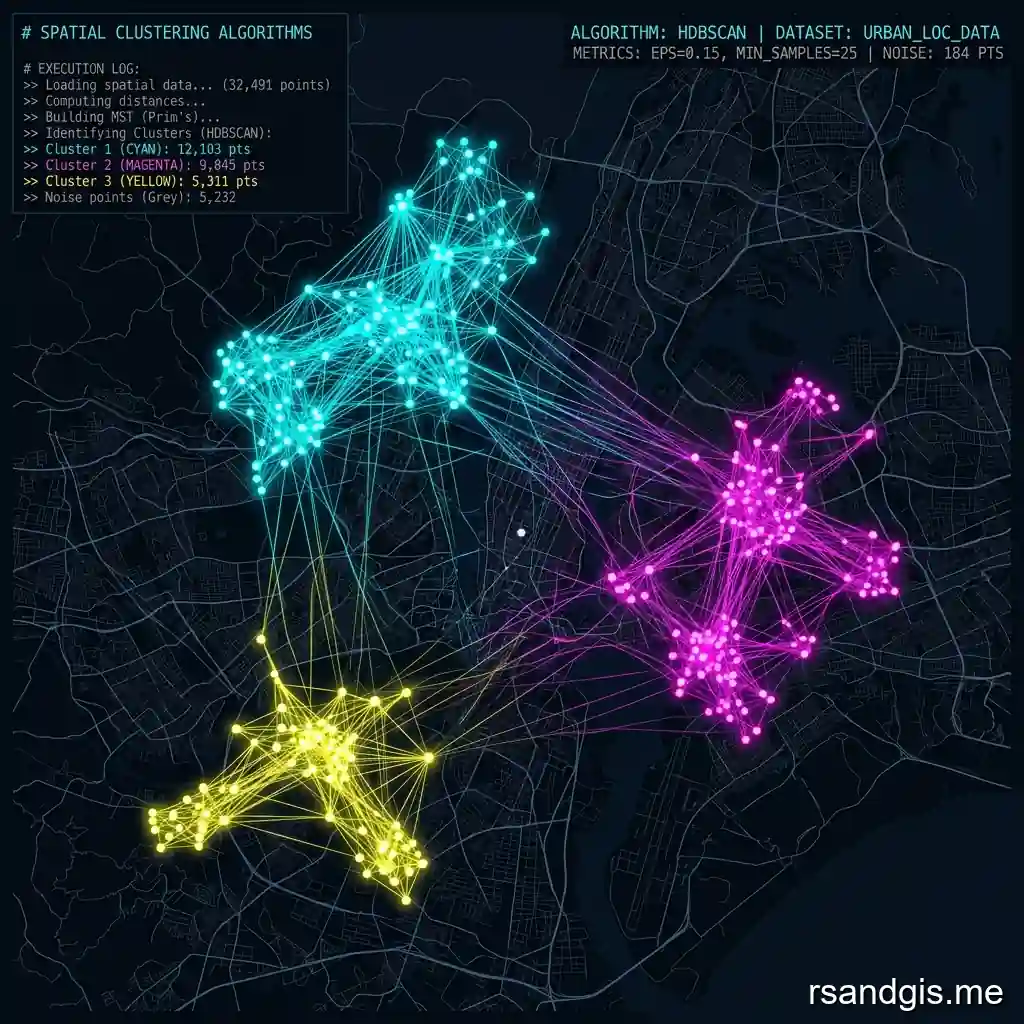
While DBSCAN is incredibly powerful, it suffers from a significant limitation: it relies on a single global density threshold (defined by `eps`). In many real-world spatial scenarios, clusters exhibit varying densities. For example, a dataset containing locations of retail stores might feature highly dense clusters in dense urban centers like Manhattan, alongside much sparser clusters in suburban or rural areas. DBSCAN struggles to identify both types of clusters simultaneously; an `eps` optimized for the city will classify the rural clusters as noise, while an `eps` optimized for the rural areas will merge distinct city clusters into one. Enter HDBSCAN, an advanced evolution of the DBSCAN algorithm that addresses this precise limitation.

The Advantages of a Hierarchical Approach

HDBSCAN transforms the density-based clustering paradigm by introducing a hierarchical component. Instead of demanding a single `eps` value, HDBSCAN explores all possible `eps` values, building a cluster hierarchy that represents the data's structure across all density scales. It then utilizes a sophisticated technique called "condensed tree extraction" to extract a flat set of clusters from this hierarchy, dynamically selecting the most stable clusters across different density levels. This allows HDBSCAN to seamlessly discover dense clusters embedded within sparse noise, as well as sparse clusters separated by even sparser noise, without requiring the user to guess the perfect `eps` parameter.

Understanding the Mutual Reachability Distance

At the core of HDBSCAN's mechanics lies the concept of mutual reachability distance. To construct the hierarchy, HDBSCAN first transforms the distance space to push anomalous, low-density points further away from the dense core. This is achieved by defining the mutual reachability distance between two points as the maximum of three values: the core distance of the first point, the core distance of the second point, and the actual distance between them. The core distance of a point is simply the distance to its k-th nearest neighbor. This transformation effectively penalizes points situated in low-density regions, ensuring they do not artificially bridge the gap between distinct, high-density clusters. By building a minimum spanning tree based on this transformed distance metric, HDBSCAN robustly captures the underlying topological structure of the geographic data.

Parameter Tuning in HDBSCAN

One of the most compelling advantages of HDBSCAN is its relative insensitivity to parameter tuning compared to its predecessor. While DBSCAN requires agonizing over the precise `eps` value, HDBSCAN largely relies on a single primary parameter: `min_cluster_size`. This parameter is highly intuitive; it simply asks the user to define the smallest grouping of points that they would consider to be a meaningful cluster. The algorithm handles the complex density estimations internally. Another parameter, `min_samples`, acts as a smoothing factor, controlling how conservative the algorithm is when deciding if a point is a core point or noise. By providing a more intuitive parameterization scheme, HDBSCAN significantly accelerates the spatial analysis workflow in Python.

Soft Clustering and Probabilities

Another profound feature of the HDBSCAN implementation in Python is its support for soft clustering. Standard DBSCAN is a hard clustering algorithm; a point either belongs to a cluster or it does not. HDBSCAN, however, can calculate the probability of a point belonging to its assigned cluster. This probabilistic framework is incredibly useful in spatial analysis, particularly at the boundaries of clusters where the transition between a cluster and noise is ambiguous. Analysts can use these probability scores to filter out low-confidence cluster assignments, leading to cleaner, more reliable insights. Points situated on the fringes of a geographic grouping will naturally receive lower probability scores, reflecting their marginal status, whereas points deeply embedded within the cluster core will receive scores approaching 1.0.

K-Means in a Geographic Context

No discussion of clustering is complete without addressing K-Means. While primarily designed for Euclidean spaces and known to struggle with non-spherical clusters and varying densities, K-Means remains a surprisingly prevalent tool in spatial analysis due to its simplicity, speed, and ease of interpretation. In specific scenarios—such as dividing a city into roughly equal service territories for delivery drivers, or placing a predetermined number of distribution centers to minimize travel distances—K-Means can be highly effective. However, applying K-Means to spatial coordinates requires significant caveats and workarounds.

The Problem with K-Means and Lat/Lon

The standard K-Means algorithm relies fundamentally on calculating the mean (centroid) of a group of points and minimizing the sum of squared Euclidean distances to these centroids. When applied directly to unprojected latitude and longitude coordinates, K-Means assumes the world is a flat cylinder. As you move further away from the equator, the physical distance represented by one degree of longitude shrinks dramatically, while the physical distance of one degree of latitude remains relatively constant. This distortion means that calculating the Euclidean mean of coordinates near the poles results in a centroid that does not accurately represent the true geographic center. Consequently, the resulting clusters become artificially skewed and elongated along the longitudinal axis, rendering the spatial partitions mathematically invalid and practically useless.

Data Projection Strategies

To responsibly utilize K-Means for spatial clustering, the geographical coordinates must first be transformed from a spherical coordinate system (lat/lon) into a projected Cartesian coordinate system using tools like PyProj or GeoPandas. A projection like the Universal Transverse Mercator (UTM) or an appropriate local state plane coordinate system mathematically flattens a specific region of the Earth, minimizing distortion for that specific area. Once the coordinates are projected into meters or feet, standard Euclidean distance calculations become valid proxies for physical distance. The K-Means algorithm can then be executed on these projected coordinates safely. After the clusters are assigned and the centroids calculated, the results can be reverse-projected back into latitude and longitude for visualization on web maps or integration with other geospatial tools.

Optimizing the Number of Clusters (K)

The defining characteristic—and often the greatest challenge—of K-Means is the requirement to specify the number of clusters (K) in advance. In many exploratory spatial analyses, the optimal number of clusters is unknown. Various heuristics exist to aid in selecting K, the most common being the Elbow Method and the Silhouette Score. The Elbow Method involves plotting the within-cluster sum of squares (inertia) against a range of K values and identifying the point where the rate of decrease sharply slows down, forming an "elbow." The Silhouette Score, conversely, measures how similar an object is to its own cluster compared to other clusters, producing a score between -1 and 1. In Python, the `yellowbrick` library provides excellent visual diagnostics to streamline the process of determining the optimal K value for spatial datasets.

Mini-Batch K-Means for Massive Datasets

When dealing with truly massive geographic datasets—such as millions of GPS pings from a fleet of vehicles—standard K-Means can become computationally intractable, taking hours to converge. To address this, Python's `scikit-learn` offers the Mini-Batch K-Means algorithm. Instead of utilizing the entire dataset at each iteration, Mini-Batch K-Means uses random subsets (mini-batches) of the data to update the centroids. This stochastic approach drastically reduces computation time while generally yielding clustering results that are only marginally inferior to the standard algorithm. For many large-scale spatial applications where approximate cluster centers are sufficient, Mini-Batch K-Means is an essential optimization technique.

Spatial Weights and Regionalization

Beyond traditional point clustering algorithms like DBSCAN and K-Means, geographic data science encompasses a broader class of techniques known as regionalization or spatially constrained clustering. These methods are essential when dealing with polygon data (e.g., census tracts, zip codes, counties) rather than individual points. The goal of regionalization is to group geographic areas into larger, contiguous regions based on the similarity of their attributes (like income, population density, or crime rates), while strictly enforcing the condition that the resulting regions must be geographically connected. This is fundamentally different from K-Means or DBSCAN, which might group a high-income neighborhood in New York with a high-income neighborhood in Los Angeles simply because their attributes are similar. Regionalization forces spatial contiguity.

Constructing Spatial Weights Matrices

The foundation of regionalization algorithms is the spatial weights matrix. This mathematical construct defines the neighborhood relationships between different geographic entities. In Python, the `PySAL` (Python Spatial Analysis Library) ecosystem is the gold standard for creating and manipulating spatial weights. The matrix represents a graph where each node is a geographic area, and edges represent spatial connectivity. There are several ways to define this connectivity. The most common is contiguity-based weights, such as Queen contiguity (regions share an edge or a vertex) or Rook contiguity (regions share only an edge). Alternatively, distance-based weights can be used, connecting regions whose centroids fall within a certain distance threshold, or using a K-Nearest Neighbors approach.

Spatially Constrained Agglomerative Clustering

One of the most powerful algorithms for regionalization available in Python is Spatially Constrained Agglomerative Clustering, implemented in `scikit-learn`. This algorithm begins with each geographic area in its own individual cluster. It then iteratively merges the two most similar clusters based on their attributes (using metrics like Ward's linkage, which minimizes the variance within the newly formed cluster). However, unlike standard hierarchical clustering, this algorithm incorporates a connectivity matrix (derived from the spatial weights). The algorithm is restricted to only merging clusters that are spatially adjacent according to the connectivity matrix. This ensures that the final aggregated regions are always geographically contiguous, making it an invaluable tool for drawing political districts, defining sales territories, or creating custom geographic reporting units.

Max-P Regions Problem

Another sophisticated regionalization technique provided by the PySAL ecosystem is the Max-P regions algorithm. This algorithm is designed to solve a complex optimization problem: group areas into an unknown maximum number of regions (P), such that each region satisfies a minimum threshold for a specific spatially extensive attribute (such as a minimum population required for a new school district), while maximizing the internal homogeneity of the regions based on other attributes. The Max-P problem is computationally NP-hard, meaning finding the perfect solution is generally impossible for large datasets. PySAL employs heuristic approaches, such as greedy algorithms followed by simulated annealing or tabu search, to find high-quality, near-optimal solutions. This advanced technique represents the cutting edge of applied spatial clustering in Python.

Evaluating Regionalization Quality

Evaluating the quality of regionalization results requires different metrics than point clustering. Since the goal is often to maximize internal homogeneity while maintaining spatial contiguity, metrics like the Spatial Pseudo F-Statistic are employed. This statistic compares the variance of the attributes within the formed regions to the variance between the regions. A higher Pseudo F-Statistic indicates that the regions are internally cohesive and distinct from one another. Visual inspection remains a critical component; generating choropleth maps of the resulting regions using libraries like `geopandas` and `matplotlib` allows analysts to intuitively assess whether the algorithmic outputs align with logical geographic boundaries and real-world domain constraints.

Integrating Clustering with Machine Learning Pipelines

The true power of spatial clustering algorithms in Python is unlocked when they are integrated into broader machine learning pipelines. Clusters themselves are rarely the final output; rather, cluster assignments often serve as engineered features for downstream predictive models. For instance, the cluster ID assigned to a house based on its location can be a highly predictive categorical feature in a real estate pricing model, capturing unquantifiable neighborhood characteristics that raw latitude and longitude fail to convey. Scikit-learn's pipeline architecture seamlessly allows spatial clustering steps to be chained with data scaling, feature extraction, and predictive estimators like Random Forests or Gradient Boosting Machines.

Feature Engineering with Spatial Context

When incorporating spatial cluster labels into a machine learning model, one must handle them carefully. Since cluster IDs are categorical variables without inherent numerical ordering, they should generally be one-hot encoded before being fed into algorithms like linear regression or neural networks. Tree-based models can sometimes handle categorical variables directly, but encoding is often preferred for consistency. Furthermore, calculating the distance from a data point to the centroid of its assigned cluster, or the distance to the centroids of all clusters, can provide powerful continuous features that capture the point's relative position within the geographic topology, significantly boosting the predictive accuracy of complex spatial models.

Challenges in Production Deployments

Deploying spatial clustering algorithms to production environments introduces a unique set of challenges. Algorithms like DBSCAN and Agglomerative Clustering are transductive, meaning they cannot easily assign new, unseen data points to existing clusters without recalculating the entire clustering structure. This is highly problematic for real-time applications, such as assigning a user to a delivery zone based on their current GPS coordinates. To overcome this, developers often use a hybrid approach: they run the complex spatial clustering algorithm periodically offline to generate the clusters, and then train a supervised classification model (like K-Nearest Neighbors or a Support Vector Machine) to predict the cluster labels for new points in real-time. This provides the sophisticated geographic groupings of spatial clustering with the millisecond latency required for production systems.

The Future of Spatial Clustering

The landscape of spatial clustering algorithms in Python is continuously evolving. The integration of deep learning techniques, such as Graph Neural Networks (GNNs), offers promising new avenues for capturing complex, non-linear spatial relationships that traditional algorithms might miss. Additionally, as the volume of real-time streaming spatial data increases, the development of robust, online spatial clustering algorithms that can continuously update cluster definitions without massive recalculations will become increasingly critical. The Python ecosystem, with its vibrant open-source community and unparalleled array of scientific libraries, remains perfectly positioned at the forefront of this geographic data science revolution, providing the tools necessary to decode the complex spatial patterns shaping our world.

Conclusion

Mastering the application and theoretical underpinnings of these algorithms is not merely an academic exercise; it is a practical necessity for anyone seeking to extract maximum value from location-based data. By understanding the nuances of distance metrics, the strengths and limitations of DBSCAN, HDBSCAN, and K-Means, and the power of spatially constrained regionalization, data scientists can unlock profound insights hidden within geographic datasets. The combination of Python's robust libraries and a deep comprehension of spatial principles provides an unparalleled framework for tackling the most complex and demanding geospatial challenges of the modern era.