Satellite Based Soil Moisture Monitoring Techniques

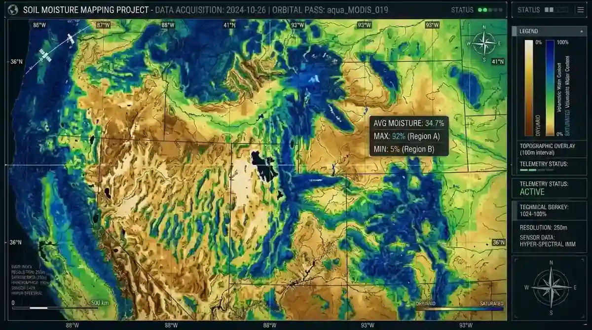
rsandgis.me

The practice of satellite based soil moisture monitoring represents a critical convergence of microwave physics, orbital mechanics, and advanced computational algorithms, providing essential data for climatology, agriculture, and hydrology. At its core, estimating the water content of the Earth's topsoil from hundreds of kilometers in space relies on the fundamental interaction between electromagnetic radiation and the dielectric properties of water and soil matrices. As global climate patterns become increasingly erratic, the demand for high-resolution, temporally frequent soil moisture datasets has driven rapid advancements in both active and passive remote sensing technologies. This article explores the technical foundations, prominent satellite missions like SMAP, SMOS, and Sentinel-1, the underlying retrieval algorithms, and practical Python implementations for processing these complex datasets.

Introduction to Microwave Remote Sensing for Soil Moisture

Optical and infrared remote sensing techniques are largely ineffective for soil moisture estimation because they cannot penetrate cloud cover and are extremely sensitive to atmospheric atmospheric scattering. Furthermore, they only capture the absolute surface skin temperature or reflectance. In contrast, microwave remote sensing, operating at frequencies between 1 GHz and 100 GHz (wavelengths from 30 cm to 0.3 cm), offers unique advantages for terrestrial observation. The microwave spectrum is largely transparent to the atmosphere, allowing for all-weather, day-and-night continuous monitoring. More importantly, longer microwave wavelengths, particularly in the L-band (1-2 GHz) and C-band (4-8 GHz), can penetrate vegetation canopies and probe the top few centimeters of the soil column.

The Physical Basis: Dielectric Constant

The entire premise of satellite based soil moisture monitoring hinges on the large contrast between the relative dielectric constant (permittivity) of dry soil and that of liquid water at microwave frequencies. The relative dielectric constant is a complex number comprising a real part (related to the ability of the material to store electrical energy) and an imaginary part (related to energy loss or absorption). At L-band frequencies (~1.4 GHz), the real part of the dielectric constant for dry soil typically ranges from 2 to 4. In stark contrast, the real part of the dielectric constant for pure liquid water is approximately 80 at room temperature.

When water is introduced to a dry soil matrix, the effective dielectric constant of the bulk soil-water-air mixture increases dramatically. This relationship is not strictly linear due to the bound water fraction—water molecules tightly held to soil particles by matric forces, which exhibit restricted rotational freedom and thus a lower dielectric constant than free water. Semi-empirical dielectric mixing models, such as the Dobson model or the Mironov model, are utilized to relate the volumetric soil moisture (expressed in cm³/cm³) to the complex dielectric constant of the soil. The resulting dielectric constant directly governs the emissivity (for passive radiometers) and the radar backscatter coefficient (for active radars) of the land surface.

Leading Satellite Missions for Soil Moisture

Over the past two decades, space agencies worldwide have launched specialized satellite missions dedicated to mapping global soil moisture. These missions utilize either passive radiometry, active radar, or a combination of both to achieve various trade-offs between spatial resolution and temporal revisit times.

Soil Moisture Active Passive (SMAP)

Launched by NASA in January 2015, the Soil Moisture Active Passive (SMAP) observatory was designed to provide the highest-resolution, most accurate global soil moisture maps ever produced. SMAP originally featured two L-band instruments sharing a single 6-meter spinning deployable mesh reflector antenna: a radiometer (passive) operating at 1.41 GHz and a Synthetic Aperture Radar (SAR, active) operating at 1.26 GHz. The radiometer provides high-accuracy but coarse-resolution (~40 km) data, measuring the naturally emitted thermal radiation from the Earth's surface in horizontal (H) and vertical (V) polarizations. The radar was designed to provide high-resolution (1-3 km) but noisier backscatter measurements. Although the SMAP radar experienced an unrecoverable hardware failure in July 2015, the radiometer continues to function flawlessly, providing exceptional data. To compensate for the loss of its own radar, SMAP currently employs data fusion techniques, integrating C-band SAR data from the Copernicus Sentinel-1 satellites to produce a downscaled, high-resolution soil moisture product (SMAP/Sentinel-1 L2_SM_SP).

Soil Moisture and Ocean Salinity (SMOS)

The European Space Agency's (ESA) Soil Moisture and Ocean Salinity (SMOS) mission, launched in 2009, takes a radically different engineering approach. SMOS utilizes an L-band (1.4 GHz) 2D interferometric radiometer known as MIRAS (Microwave Imaging Radiometer using Aperture Synthesis). Instead of a large rotating physical antenna like SMAP, MIRAS consists of 69 small antenna elements distributed along three deployable arms forming a Y-shape. By cross-correlating the signals received by these spatially separated antennas, SMOS synthesizes a large aperture electronically, achieving a spatial resolution of roughly 35-50 km. SMOS observes the Earth at multiple incidence angles (from 0 to 55 degrees) as the satellite passes overhead. This multi-angular, fully polarimetric capability provides rich information that helps disentangle the effects of soil moisture from vegetation opacity and surface roughness during the retrieval process.

Sentinel-1 and Synthetic Aperture Radar (SAR)

While missions like SMOS and SMAP focus on L-band radiometry for high accuracy, they suffer from coarse spatial resolution. The European Copernicus Sentinel-1 mission addresses the need for high-resolution monitoring. Sentinel-1 is a constellation of two satellites (Sentinel-1A and 1B, though 1B ended its mission in 2022 and awaits replacement by 1C) carrying a C-band (5.405 GHz) SAR instrument. SAR techniques process the Doppler history of radar echoes as the satellite moves to synthesize a virtually long antenna, yielding spatial resolutions on the order of 10 to 20 meters.

However, C-band SAR is highly sensitive to vegetation structure, surface roughness, and topography, making direct soil moisture retrieval challenging. To extract soil moisture from Sentinel-1 backscatter, researchers typically employ change detection algorithms. These algorithms assume that surface roughness and vegetation change slowly compared to soil moisture. By normalizing the current backscatter against historical dry and wet references for a given pixel, a relative soil wetness index can be calculated, which is then scaled to absolute volumetric soil moisture.

Soil Moisture Retrieval Algorithms

Translating raw satellite measurements—such as brightness temperature (radiometer) or backscatter cross-section (radar)—into volumetric soil moisture requires sophisticated physical models that invert the radiative transfer equations.

Passive Microwave Retrieval Algorithms (Tau-Omega Model)

For passive L-band radiometers like SMAP and SMOS, the standard approach is based on the zeroth-order solution to the radiative transfer equation, commonly known as the Tau-Omega (τ-ω) model. A radiometer measures the brightness temperature (Tb) of the Earth, which is the product of the physical temperature of the emitting medium and its microwave emissivity.

The Tau-Omega model conceptualizes the land surface as a rough soil boundary covered by a vegetation layer. The brightness temperature observed by the satellite is the sum of three main components: 1. The direct emission from the vegetation canopy. 2. The emission from the soil surface that is attenuated as it passes through the vegetation canopy. 3. The downward emission from the vegetation that is reflected by the soil surface and then attenuated again by the canopy as it travels upward towards the satellite sensor.

The model requires several critical parameters: the vegetation optical depth (tau, τ), which quantifies the attenuation of the microwave signal by the canopy; the single scattering albedo (omega, ω), which accounts for the scattering of microwave radiation within the canopy; and the soil surface roughness parameter (h). Once the effects of vegetation and roughness are modeled and removed, the smooth-surface soil emissivity is isolated. Using the physical temperature of the soil (often derived from ancillary numerical weather prediction models), the effective dielectric constant is calculated. Finally, a dielectric mixing model is inverted to yield the volumetric soil moisture.

Active Microwave Retrieval Algorithms

Retrieving soil moisture from active radar backscatter (σ°) is fundamentally more complex due to the coherent nature of the radar signal, which is highly sensitive to the geometric structure of the scattering surface (roughness) and volume (vegetation). Forward scattering models, such as the Integral Equation Model (IEM) or the Advanced Integral Equation Model (AIEM), simulate the expected radar backscatter given a set of soil moisture, roughness, and incidence angle parameters.

Because multiple combinations of soil moisture and roughness can produce the same backscatter value, this inversion is an ill-posed problem. Solutions involve using time-series approaches like the TU Wien change detection method, which relies on defining historical dry and wet limits for each pixel. Another approach utilizes machine learning architectures, such as Artificial Neural Networks (ANNs) or Support Vector Machines (SVMs), trained on large datasets generated by physical scattering models (like the Water Cloud Model) to map the non-linear relationship between SAR backscatter, vegetation indices (like NDVI), and soil moisture directly.

Processing Satellite Data with Python

Working with satellite based soil moisture monitoring data requires programmatic approaches to handle massive netCDF or HDF5 files, perform spatial reprojections, and execute time-series analysis. Python, with its rich ecosystem of geospatial libraries, is the industry standard for this task.

Accessing and Analyzing SMAP Data with Xarray

NASA provides SMAP data through the National Snow and Ice Data Center (NSIDC) DAAC. The data is commonly distributed in HDF5 format. The `xarray` library in Python is exceptionally well-suited for handling these multi-dimensional arrays.

Below is a technical example demonstrating how to load a SMAP Level-3 global daily soil moisture product, apply data quality masks, and visualize the output using `xarray` and `matplotlib`.

import xarray as xr
import matplotlib.pyplot as plt
import numpy as np

# Load SMAP L3 Radiometer Global Daily 36 km EASE-Grid Soil Moisture
# File path would point to a locally downloaded HDF5 file
file_path = 'SMAP_L3_SM_P_20260823_R18290_001.h5'

# Open the HDF5 file using xarray with the h5netcdf engine
# SMAP data groups are structured; we access the 'Soil_Moisture_Retrieval_Data' group
ds = xr.open_dataset(file_path, group='Soil_Moisture_Retrieval_Data', engine='h5netcdf')

# Extract the soil moisture variable and the retrieval quality flag
soil_moisture = ds['soil_moisture']
retrieval_qual_flag = ds['retrieval_qual_flag']

# The quality flag is a bitmask. For SMAP, a value of 0 indicates recommended quality.
# We create a mask to filter out unreliable pixels (e.g., dense vegetation, frozen soil, RFI)
valid_data_mask = (retrieval_qual_flag == 0)

# Apply the mask and handle fill values (typically -9999.0)
sm_clean = soil_moisture.where(valid_data_mask)
sm_clean = sm_clean.where(sm_clean != -9999.0)

# Plotting the global map
plt.figure(figsize=(12, 6))
# xarray automatically handles the 2D plotting based on array dimensions
sm_clean.plot(
    cmap='viridis_r', 
    vmin=0.0, 
    vmax=0.5,
    cbar_kwargs={'label': 'Volumetric Soil Moisture (cm³/cm³)'}
)
plt.title('SMAP L3 Global Soil Moisture - August 23, 2026')
plt.xlabel('EASE-Grid X (Longitude index)')
plt.ylabel('EASE-Grid Y (Latitude index)')
plt.tight_layout()
plt.show()

This code snippet illustrates the necessity of applying bitmask quality flags; failing to filter out pixels affected by radio frequency interference (RFI) or urban infrastructure will lead to heavily skewed environmental analyses.

Sentinel-1 Soil Moisture Estimation using Google Earth Engine (GEE)

Downloading and processing terabytes of Sentinel-1 SAR imagery locally is computationally prohibitive for broad-scale analysis. Google Earth Engine (GEE) provides a cloud-based platform to access and process this data on the fly. Python users can interact with GEE using the `earthengine-api` package.

The following snippet outlines the logic for a basic change detection algorithm applied to Sentinel-1 backscatter to estimate a relative soil moisture index, leveraging GEE's server-side processing capabilities.

import ee

# Initialize the Earth Engine API
ee.Initialize()

# Define the Area of Interest (AOI) - e.g., an agricultural region in California
aoi = ee.Geometry.Rectangle([-120.5, 36.5, -119.5, 37.5])

# Define the date range for observation and historical baseline
target_date_start = '2026-08-01'
target_date_end = '2026-08-31'
historical_start = '2020-01-01'

# Load Sentinel-1 GRD collection, filtering for VV polarization and descending passes
s1_collection = ee.ImageCollection("COPERNICUS/S1_GRD") \
    .filterBounds(aoi) \
    .filter(ee.Filter.listContains('transmitterReceiverPolarisation', 'VV')) \
    .filter(ee.Filter.eq('orbitProperties_pass', 'DESCENDING')) \
    .filter(ee.Filter.eq('instrumentMode', 'IW')) \
    .select('VV')

# Calculate the historical minimum (dry state) and maximum (wet state) backscatter
s1_historical = s1_collection.filterDate(historical_start, target_date_start)
sigma_min = s1_historical.min()
sigma_max = s1_historical.max()

# Get the mean backscatter for the target month
s1_target = s1_collection.filterDate(target_date_start, target_date_end).mean()

# Calculate the relative Soil Moisture Index (SMI)
# SMI = (Sigma_target - Sigma_min) / (Sigma_max - Sigma_min)
smi = s1_target.subtract(sigma_min).divide(sigma_max.subtract(sigma_min))

# Clamp values between 0 and 1 to handle anomalies
smi = smi.clamp(0, 1)

# At this stage, the 'smi' image is an Earth Engine object ready to be exported
# or visualized in a folium map or GEE App.

While this change detection model is simplified—it assumes vegetation opacity remains constant—it forms the conceptual bedrock for more advanced active microwave retrieval architectures operating within cloud computing environments.

Challenges and Future Directions

Despite significant technological leaps, satellite based soil moisture monitoring continues to face profound scientific and engineering challenges. The accuracy of global datasets is heavily dependent on auxiliary parameters and the successful mitigation of signal contamination.

Vegetation Scattering and Surface Roughness

The most persistent challenge in microwave remote sensing of soils is the presence of vegetation. As biomass increases, the vegetation canopy severely attenuates the microwave emission from the soil and introduces its own emission and scattering components. In dense forests (where vegetation water content exceeds 5 kg/m²), L-band radiometry becomes entirely opaque to the soil surface, rendering retrieval algorithms useless. To combat this, researchers are exploring the P-band frequency (around 435 MHz), which boasts significantly deeper penetration capabilities. The ESA BIOMASS mission, planned for launch in the near future, will carry a P-band SAR that could revolutionize sub-canopy soil moisture observation, although its primary mandate is forest biomass mapping.

Surface roughness presents another major confounding variable. In agricultural regions, plowing and tilling create highly structured roughness patterns that alter the emission and scattering angles of microwave energy. Current global models rely on static or semi-static roughness maps, which fail to capture rapid anthropogenic changes to the soil structure. Incorporating dynamic roughness models, potentially informed by high-resolution optical data or multi-angular SAR, is a primary focus of ongoing algorithm development.

High-Resolution Downscaling

Hydrological modeling at the watershed scale and precision agriculture require soil moisture data at spatial resolutions of 100 meters or finer. Passive radiometers like SMAP provide 36 km resolution, which is highly accurate but practically useless for farm-level decision-making. Therefore, downscaling methodologies are critical.

Thermal inertial methods represent a prominent downscaling technique. These methods fuse coarse-resolution microwave data with high-resolution land surface temperature (LST) and normalized difference vegetation index (NDVI) data from optical satellites (like MODIS or Landsat). Because wet soil has a higher heat capacity than dry soil, it exhibits a smaller diurnal temperature amplitude. By analyzing the relationship between LST, NDVI, and coarse-scale soil moisture, algorithms can disaggregate the microwave signal into higher-resolution grids. Furthermore, deep learning techniques, such as Convolutional Neural Networks (CNNs) and Generative Adversarial Networks (GANs), are increasingly being trained to execute non-linear spatial downscaling, learning complex spatial patterns from disparate sensor arrays to output synthesized sub-kilometer soil moisture fields.

Conclusion

The science of satellite based soil moisture monitoring is an indispensable asset for understanding the Earth's hydrological cycle and managing agricultural resources in the face of climate instability. Through the continuous operation of L-band missions like SMAP and SMOS, combined with the high-resolution capabilities of Sentinel-1 C-band SAR, the global scientific community possesses unprecedented visibility into the terrestrial water balance. As algorithmic paradigms shift toward machine learning integrations and multi-sensor data fusion—managed programmatically via Python ecosystems like xarray and Google Earth Engine—the precision, resolution, and utility of soil moisture datasets will continue to accelerate. Overcoming the physical limitations imposed by dense vegetation and heterogeneous surface roughness will require next-generation sensor technologies, ensuring that spaceborne hydrological observation remains a dynamic and vital frontier of remote sensing.

Frequently Asked Questions