Guide to Drone Based Lidar Mapping Accuracy

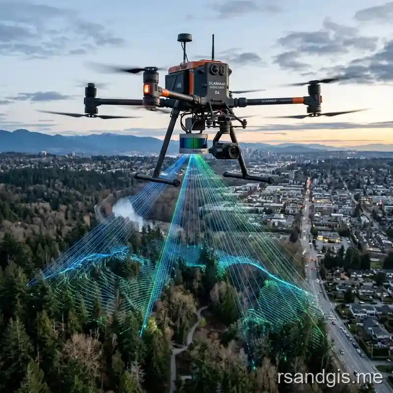
Achieving optimal drone based lidar mapping accuracy requires a comprehensive understanding of the intricate error budgets inherent in UAV-mounted laser scanning systems. In the realm of contemporary remote sensing and geospatial analytics, the deployment of Unmanned Aerial Vehicles (UAVs) equipped with Light Detection and Ranging (LiDAR) sensors has revolutionized topographical mapping. However, the exactitude of the generated point clouds is not solely a function of the laser's innate precision; rather, it is the culmination of a highly complex integration between the laser scanner, the Global Navigation Satellite System (GNSS), the Inertial Measurement Unit (IMU), and the rigorous post-processing algorithms applied to the raw data. As professionals push the boundaries of surveying from the air, examining the multifarious variables that degrade or enhance measurement fidelity becomes essential for delivering engineering-grade deliverables.

Introduction to UAV LiDAR System Metrics

Before dissecting the specific components that influence system performance, it is imperative to establish the fundamental metrics used to evaluate the quality of aerial survey data. The theoretical limits of the hardware often differ significantly from the empirical results observed in the field, primarily due to dynamic environmental conditions and mechanical vibrations induced by the drone's propulsion system.

Defining Absolute and Relative Precision

In geospatial sciences, precision and accuracy are distinct yet interdependent concepts. Relative precision refers to the internal consistency of the point cloud—how well individual laser returns align with one another within the same dataset. This is highly dependent on the IMU's high-frequency noise and the laser scanner's ranging noise. Conversely, absolute accuracy defines the alignment of the point cloud relative to a known global coordinate reference system (CRS). Achieving high absolute accuracy necessitates robust GNSS positioning, accurate base station coordinates, and precise lever-arm measurements between the GNSS antenna and the optical center of the LiDAR sensor. A dataset can possess exquisite relative precision, exhibiting crisp edges on building structures, while simultaneously suffering from poor absolute accuracy if it is uniformly shifted by several meters from its true geographic position.

The Error Budget in Aerial Topography

The concept of an error budget is fundamental to understanding spatial data quality. An error budget aggregates the individual uncertainties of all subsystems—GNSS, IMU, laser ranging, and boresight calibration—to estimate the maximum expected deviation of a computed 3D point. Because these subsystems are mathematically coupled through the direct georeferencing equation, an angular error in the IMU propagates into a positional error that scales linearly with the flying altitude (Above Ground Level, AGL).

Systematic vs. Random Errors

Errors within the budget are broadly classified as systematic or random. Random errors, such as thermal noise in the laser detector or phase noise in the GNSS receiver, follow a Gaussian distribution and can often be mitigated through averaging or high point density. Systematic errors, however, introduce a consistent bias. Examples include an incorrectly measured lever arm, uncalibrated boresight misalignment, or a constant atmospheric refraction offset. Systematic errors cannot be eliminated through oversampling; they must be mathematically modeled and removed during the post-processing phase or calibration flights.

Sensor Integration and Calibration Effects

The foundation of direct georeferencing relies on the seamless integration of the Position and Orientation System (POS). The POS consists of the GNSS receiver (providing translation) and the IMU (providing rotation). Any desynchronization or miscalibration between these components directly degrades the output geometry.

Inertial Measurement Unit (IMU) Imperfections

The IMU is arguably the most critical and cost-determining component in a drone-based mapping payload. Unlike terrestrial scanning where the sensor is static, a drone is constantly subjected to pitch, roll, and yaw perturbations. The IMU must sample these angular rates and linear accelerations at extremely high frequencies (typically 200 Hz to 500 Hz) to maintain an accurate estimate of the sensor's attitude between low-frequency (1 Hz to 10 Hz) GNSS updates.

Gyroscope Drift and Accelerometer Bias

Micro-Electro-Mechanical Systems (MEMS) IMUs, commonly used on drones due to their light weight, are susceptible to gyroscope drift and accelerometer bias. Gyroscope drift refers to the integration of angular rate noise over time, which manifests as a slowly increasing angular error. If the drone loses GNSS lock, the system relies purely on the IMU (dead reckoning), and this drift rapidly corrupts the trajectory. Advanced Kalman filters are employed in processing software to estimate and continuously zero out these biases whenever GNSS data is available, a process known as tight coupling.

Global Navigation Satellite System (GNSS) Limitations

While RTK and PPK technologies offer centimeter-level positional accuracy under ideal conditions, the dynamic nature of a drone flight introduces specific GNSS vulnerabilities. The receiver must maintain continuous phase lock on carrier waves from multiple satellite constellations (GPS, GLONASS, Galileo, BeiDou).

Multipath Effects and Ionospheric Delay

Multipath occurs when satellite signals bounce off reflective surfaces (such as nearby buildings or even parts of the drone's airframe) before reaching the antenna. This creates a phase delay that the receiver misinterprets as a longer distance to the satellite. Although aviation-grade choke ring antennas mitigate multipath, they are too heavy for drones. Consequently, careful antenna placement and ground plane design are vital. Additionally, fluctuations in total electron content (TEC) in the ionosphere cause signal delays that must be modeled using dual-frequency (L1/L2) receivers.

Boresight Misalignment Calibration

Boresight calibration is the process of determining the exact rotational offset (roll, pitch, and heading) between the IMU's coordinate frame and the laser scanner's optical coordinate frame. Even an infinitesimal misalignment of a few millidegrees will cause severe planar discrepancies in the overlapping regions of adjacent flight strips.

Flight Patterns for Boresight Optimization

To accurately compute these angles, operators execute specific calibration flight patterns over terrain with diverse geometric features, such as pitched roofs and flat parking lots. These patterns typically involve flying overlapping lines in opposite directions, as well as crossing lines at a 90-degree angle. Specialized software algorithms analyze the discrepancies between the point clouds of the different passes to inversely calculate the boresight angles, thereby tightening the relative precision.

Laser Scanner Parameters Influencing Precision

Beyond the positioning system, the intrinsic characteristics of the laser scanner hardware play a paramount role in determining spatial resolution and ranging fidelity. The physics of laser propagation dictate the ultimate limitations of the sensor.

Pulse Rate and Footprint Diameter

The pulse repetition rate (PRR), measured in kilohertz (kHz), dictates how many laser pulses are emitted per second. While a higher PRR increases point density, it often requires dividing the available laser power, reducing the maximum effective range. The footprint diameter, determined by the beam divergence angle and flying height, represents the area illuminated by a single pulse upon striking the ground.

Beam Divergence and Point Density

A smaller beam divergence yields a smaller, more focused footprint, which is crucial for resolving fine details like power lines or distinct building edges. A large footprint can bridge adjacent surfaces (e.g., a curb and a road), returning a smeared or averaged distance that diminishes accuracy. Point density (points per square meter) is a function of PRR, flying speed, altitude, and field of view (FOV). High point density improves the statistical probability of striking desired targets and allows for more aggressive filtering of noise.

Multiple Returns and Vegetation Penetration

One of the distinct advantages of LiDAR over photogrammetry is its ability to penetrate vegetation canopies to map the bare earth. When a laser pulse encounters a semi-permeable object, such as a tree canopy, part of the energy reflects off the leaves (first return), while the remaining energy continues downward to hit lower branches or the ground (subsequent returns).

Intensity Calibration and Surface Reflectance

The accuracy of the ranging measurement is influenced by the target's reflectivity. Dark or wet surfaces absorb near-infrared laser energy, resulting in a weak return signal that is difficult for the sensor's avalanche photodiode to timestamp accurately, an effect known as range walk. Calibrating the intensity values helps in identifying surface materials and correcting for reflectivity-induced ranging anomalies.

Trajectory Processing and Post-Processing Kinematics (PPK)

The raw data collected during a flight—GNSS observations, IMU raw data, and laser ranges—must be synthesized to produce the final point cloud. The generation of a highly accurate Smooth Best Estimate of Trajectory (SBET) is the cornerstone of this process.

Real-Time Kinematic (RTK) vs. PPK

RTK relies on a continuous radio or cellular link to transmit correction data from a base station to the drone in real-time. If the data link drops, positioning falls back to standalone GNSS, severely degrading accuracy. PPK, conversely, logs all raw satellite observations on both the drone and the base station for subsequent processing. PPK is inherently more robust and typically yields higher accuracy because the trajectory can be processed both forward and backward in time, smoothing out IMU drifts and bridging GNSS outages.

Lever Arm Offsets in Tight Coupling

The physical distances between the GNSS antenna phase center, the IMU origin, and the laser firing point are known as lever arms. These must be measured to millimeter precision. In a tightly coupled processing strategy, the raw GNSS pseudoranges and carrier phases are combined directly with IMU data in a single extended Kalman filter. If the lever arms are incorrect, rotational movements of the drone will incorrectly translate into positional shifts in the calculated trajectory.

Base Station Baseline Length Dependencies

In differential GNSS processing (both RTK and PPK), accuracy degrades as the distance (baseline) between the base station and the rover (drone) increases. This is because atmospheric conditions (ionosphere and troposphere) at the base and rover begin to decorrelate.

Network RTK (VRS) Performance

To overcome baseline limitations, operators often use Network RTK or Virtual Reference Station (VRS) networks. These networks interpolate atmospheric corrections from a grid of continuous operating reference stations (CORS) to generate a virtual base station exactly at the drone's location. While highly convenient, relying on VRS can sometimes introduce interpolation errors, making local physical base stations the gold standard for high-accuracy engineering projects.

Environmental Factors and Atmospheric Propagation

The medium through which the laser travels—the atmosphere—is dynamic and heterogeneous. Environmental variables can introduce ranging errors that are difficult to model deterministically.

Atmospheric Refraction and Turbulence

As the laser pulse travels through the atmosphere, variations in air density, temperature, and pressure cause the beam to refract (bend) slightly. Furthermore, atmospheric turbulence can scatter the beam and distort the returning wavefront. While standard atmosphere models are used in processing software to calculate the speed of light accurately, localized microclimates can cause deviations from these models.

Attenuation in High Humidity

Water vapor is highly absorptive in the near-infrared spectrum utilized by most topographical LiDAR systems (typically 905nm or 1550nm). High humidity, fog, or airborne dust attenuates the laser energy, reducing the signal-to-noise ratio. This not only decreases the effective range of the sensor but also increases ranging uncertainty, leading to a "fuzzier" point cloud.

Target Surface Characteristics

The physical geometry of the surface being mapped heavily dictates the achievable precision. Flat, hard, lambertian surfaces (like concrete) yield the best results.

Slope Angle and Surface Roughness

When the laser beam strikes a steeply sloped surface, the footprint elongates. This elongation causes the return pulse to spread out in time, making it difficult for the receiver electronics to precisely identify the peak of the pulse, introducing ranging error. Similarly, surfaces with high macro-roughness scatter the beam in unpredictable ways, increasing the thickness of the resultant point cloud profile.

Software Algorithms and Point Cloud Adjustments

The transition from raw laser points to a highly accurate digital elevation model requires sophisticated algorithmic intervention. Software suites apply various heuristic and deterministic filters to refine the data.

Strip Adjustment and Point Cloud Registration

Even with excellent PPK trajectories and boresight calibration, adjacent flight lines (strips) often exhibit minor mismatches. Strip adjustment is a post-processing technique that matches geometric features (like planar surfaces and lines) in the overlap regions of adjacent strips. By minimizing the distances between these corresponding features, the software computes a localized correction (translation and rotation) for each strip, forcing them into seamless alignment.

Iterative Closest Point (ICP) Algorithms

Many strip adjustment engines utilize variants of the Iterative Closest Point (ICP) algorithm. ICP iteratively revises the rigid body transformation needed to minimize the distance between a source point cloud and a reference point cloud. Advanced implementations segment the data into planar patches to avoid false matches on vegetation or moving objects.

Ground Filtering and Digital Elevation Model (DEM) Generation

For topographical mapping, isolating the bare earth from vegetation and anthropogenic structures is critical. The accuracy of the final DEM relies heavily on the success of these ground filtering algorithms.

Cloth Simulation Filtering (CSF)

Modern approaches, such as Cloth Simulation Filtering (CSF), mathematically invert the point cloud and simulate dropping a rigid cloth over the inverted surface. The points where the cloth rests are classified as ground. The parameters of the cloth (rigidness and grid size) must be carefully tuned based on the terrain type; overly aggressive filtering can remove valid terrain features like sharp ridges, artificially degrading the accuracy of the terrain model.

Quantifying and Validating Accuracies

A dataset cannot be deemed accurate without empirical validation against independent measurements of higher accuracy. Quality assurance and quality control (QA/QC) protocols are mandatory.

Ground Control Points (GCPs) and Checkpoints

While direct georeferencing theoretically eliminates the need for Ground Control Points (GCPs) for orientation, they are frequently utilized to remove residual systematic biases (like vertical datums shifts). Checkpoints, conversely, are not used in the processing pipeline at all; they serve solely as independent truth data to evaluate the final point cloud.

Root Mean Square Error (RMSE) Calculation

The standard statistical metric for quantifying absolute accuracy is the Root Mean Square Error (RMSE). The RMSE is calculated by measuring the difference (delta) between the coordinates of the surveyed checkpoints and the corresponding interpolated elevation in the LiDAR point cloud. A low RMSE indicates high overall accuracy, but analysts must also check for systematic biases (e.g., if all errors are in the positive direction) and maximum absolute errors (outliers).

Compliance with ASPRS Positional Accuracy Standards

In North America, the American Society for Photogrammetry and Remote Sensing (ASPRS) Positional Accuracy Standards for Digital Geospatial Data govern the reporting of spatial accuracy. These standards dictate the number and distribution of checkpoints required and provide specific thresholds for different accuracy classes based on the intended contour interval.

Vertical Data Assessment and Reporting

When reporting according to ASPRS standards, accuracy is typically expressed at a 95% confidence level. This requires verifying that the errors are normally distributed. In areas of dense vegetation, the vertical accuracy is often reported separately as Supplemental Vertical Accuracy (SVA), recognizing that non-vegetated areas (Non-Vegetated Vertical Accuracy, NVA) will inherently possess higher precision.

Future Innovations Enhancing Performance

The hardware and software landscape surrounding UAV LiDAR is rapidly evolving, driving continuous improvements in miniaturization, cost-efficiency, and spatial fidelity.

Solid-State LiDAR and Micro-Electro-Mechanical Systems (MEMS)

Traditional spinning mirror laser scanners are highly accurate but heavy and delicate. The emergence of solid-state LiDAR, utilizing Optical Phased Arrays (OPA) or MEMS mirrors, eliminates moving parts. This drastically reduces weight and increases mechanical reliability, although current generations still grapple with limited range and wider beam divergence compared to their mechanical counterparts.

Miniaturization vs. Beam Divergence

As payload weight limits decrease, manufacturers are forced to compromise on optical aperture size. A smaller aperture fundamentally limits how tightly the laser beam can be focused due to the diffraction limit. Overcoming the physical trade-off between payload weight and beam divergence remains a primary engineering challenge for next-generation lightweight systems.

Artificial Intelligence in Outlier Removal

Machine learning, particularly deep neural networks, is revolutionizing point cloud classification. Algorithms are being trained to automatically identify and classify complex features, moving beyond simple geometric filtering.

Deep Learning for Dynamic Object Filtering

One of the most persistent issues in point cloud accuracy is the presence of dynamic objects like moving cars, pedestrians, or wind-blown foliage. Deep learning models, using semantic segmentation architectures like PointNet++, can now effectively recognize and remove these transient artifacts, producing a cleaner, more reliable representation of the static environment without extensive manual editing.

Conclusion

Mastering the complexities of drone-based LiDAR systems involves a delicate balancing act across hardware configuration, flight planning execution, and rigorous data post-processing. As we have explored, the ultimate accuracy is not governed by a single metric but is instead the result of an exhaustive error budget encompassing IMU drift, GNSS precision, laser physics, and atmospheric conditions. By understanding and meticulously managing these interrelated factors, geospatial professionals can confidently harness UAV LiDAR technology to produce surveying deliverables of unprecedented detail and reliability, pushing the boundaries of what is achievable in modern cartography and topographical mapping.