QGIS Automated Geological Mapping Workflows

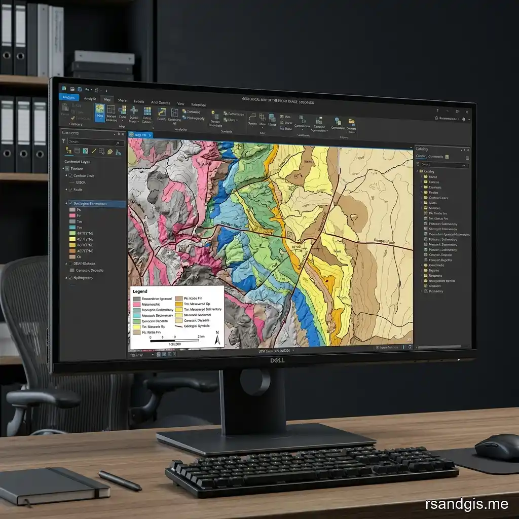
Mastering QGIS automated geological mapping workflows is essential for modern geoscientists looking to streamline spatial data analysis. In the ever-evolving landscape of geospatial technology, the ability to automate repetitive tasks is not just a luxury—it is a fundamental requirement for maintaining accuracy, efficiency, and scalability in geological surveying. Geological mapping has traditionally been a highly manual, labor-intensive process requiring field geologists to meticulously record strike and dip measurements, identify lithological boundaries, and manually digitize these features into a Geographic Information System (GIS). Today, however, the paradigm has shifted dramatically. With the advent of advanced computational algorithms, machine learning integrations, and powerful open-source platforms like Quantum GIS (QGIS), the era of manual digitization is rapidly giving way to highly sophisticated automated workflows.

The Foundations of Automating Geological Processes

Understanding QGIS automated geological mapping workflows begins with a deep dive into the theoretical and practical foundations of geographic information science. Geological mapping inherently involves the synthesis of diverse datasets: digital elevation models (DEMs), multispectral satellite imagery, aeromagnetic surveys, radiometric data, and ground-truth field observations. When performed manually, integrating these datasets is prone to human error and subjective interpretation. Automation standardizes this process, ensuring that the extraction of geological lineaments, the classification of lithological units, and the generation of structural contours are performed consistently across vast regional datasets. QGIS, as a premier open-source GIS software suite, provides an unparalleled ecosystem for building these automated pipelines through its native Model Builder, its robust Python API (PyQGIS), and its seamless integration with external processing engines such as GRASS GIS, SAGA GIS, and the Orfeo ToolBox (OTB).

The primary objective of automating these workflows is to reduce the time spent on data preprocessing and mechanical digitization, thereby freeing geoscientists to focus on higher-level structural interpretation and resource evaluation. For instance, in mineral exploration, rapid delineation of alteration zones using automated band-ratio algorithms on Landsat 8 or Sentinel-2 imagery can significantly narrow down target areas before deploying costly field crews. Similarly, in hydrogeology, automated mapping of fracture networks and fault systems using DEM derivatives (such as slope, aspect, and curvature) is critical for modeling groundwater flow in fractured rock aquifers. The sheer volume of high-resolution geospatial data available today necessitates the adoption of QGIS automated geological mapping workflows.

Data Acquisition and Preprocessing Pipelines

The first critical step in any QGIS automated geological mapping workflows is the automated acquisition and preprocessing of raw geospatial data. Raw satellite imagery and elevation models often contain artifacts, atmospheric interference, or sensor noise that must be corrected before any meaningful geological feature extraction can occur. In QGIS, these preprocessing steps can be chained together using the Graphical Modeler.

Automating DEM Hydrological and Topographical Corrections

Digital Elevation Models (DEMs) are the backbone of structural geological mapping. Automated workflows often begin by filling sinks and removing depressions in the DEM to ensure continuous flow paths—a process easily automated using the SAGA "Fill Sinks" algorithm within a QGIS model. Once the DEM is hydro-logically corrected, the workflow automatically generates derivative products: slope maps, aspect maps, hillshades at multiple illumination angles, and topographic wetness indices. Multi-directional hillshading is particularly valuable for identifying subtle structural lineaments that might be obscured by single-source illumination. By chaining these tools in QGIS, a user can input a raw DEM and automatically generate a comprehensive suite of topographical layers in minutes, a process that would manually take hours.

Multispectral Image Calibration and Band Math Automation

For lithological discrimination, multispectral imagery (e.g., Sentinel-2, ASTER, Landsat) must be converted from Digital Numbers (DN) to Top of Atmosphere (TOA) reflectance, and subsequently to Surface Reflectance (SR). While visible and near-infrared bands can use simpler algorithms like DOS1, SWIR bands (critical for geology) require rigorous radiative transfer modeling (like FLAASH or QUAC) to correct for water vapor absorption. Through QGIS automated geological mapping workflows, this radiometric calibration can be scripted via PyQGIS. Following calibration, the workflow can automatically execute a series of Raster Calculator expressions to generate geological indices. For example, the automated calculation of the Iron Oxide Ratio (Red/Blue), the Clay Mineral Ratio (SWIR1/SWIR2), and the Ferrous Minerals Ratio (SWIR/NIR) provides immediate visual highlighting of specific mineral assemblages. An automated pipeline ensures these complex map algebra equations are executed flawlessly across multiple satellite tiles without manual formula entry.

Advanced Lithological Classification Techniques

Once the data is preprocessed, the next phase of QGIS automated geological mapping workflows is the actual classification of rock types and surface materials. Traditional geological mapping relies heavily on manual polygon digitization. Automated workflows replace this with pixel-based and object-based image analysis (OBIA).

Unsupervised and Supervised Machine Learning in QGIS

QGIS seamlessly integrates with machine learning libraries through plugins like Dzetsaka or via Python scripting with Scikit-Learn. An automated workflow can be designed to ingest a stack of raster layers (e.g., DEM, slope, PCA bands, and specific mineral ratios) and perform an unsupervised K-Means or ISODATA clustering to delineate distinct lithological domains. For more precise mapping, supervised classification algorithms such as Random Forest (RF) or Support Vector Machines (SVM) are employed. In an automated QGIS workflow, the user simply provides a vector shapefile containing training polygons (ground-truth data points representing known rock types), and the script automatically trains the RF classifier, applies the model to the entire raster stack, and outputs a classified lithological map. The workflow can even automate the generation of a confusion matrix to assess the accuracy of the classification.

Object-Based Image Analysis (OBIA) Integration

While pixel-based classification is powerful, it often results in the "salt-and-pepper" effect, producing fragmented geological units that do not reflect continuous real-world stratigraphy. OBIA overcomes this by segmenting the image into homogeneous objects before classification. In QGIS, the Orfeo ToolBox (OTB) provides robust segmentation algorithms like Large Scale Mean Shift (LSMS). An advanced QGIS automated geological mapping workflows will automatically run LSMS segmentation on the multispectral imagery, calculate statistical zonal attributes (mean, variance, texture) for each resulting polygon based on the underlying raster data, and then classify these vector polygons using a machine learning algorithm. This produces clean, continuous geological units that closely resemble traditional, hand-drawn geological maps, entirely through an automated pipeline.

Comprehensive Case Study: Automating Porphyry Copper Exploration

To fully grasp the power of {keyword}, it is instructive to examine a real-world application: regional exploration for porphyry copper deposits. Porphyry systems are characterized by extensive, zoned hydrothermal alteration halos. Mapping these alteration zones manually across a 10,000 square kilometer concession using traditional field methods would take years and immense financial resources. By implementing an automated QGIS pipeline, exploration geologists can rapidly identify high-priority targets in a matter of days.

Step 1: Automated Ingestion of ASTER Data

The workflow begins with a PyQGIS script designed to automatically connect to the NASA Earthdata API, query the spatial extent of the exploration concession, and download all cloud-free ASTER Level 1T (precision terrain corrected) satellite scenes. ASTER is the premier satellite sensor for this task due to its six specific bands in the SWIR spectrum, which are critical for discriminating between phyllic, argillic, and propylitic alteration zones.

Once downloaded, the QGIS workflow automatically mosaics the individual scenes into a single, seamless regional raster dataset. Because standard empirical corrections like DOS fail in the SWIR spectrum, the script specifically pulls the pre-processed AST_07XT Surface Reflectance product. This bypasses atmospheric water vapor absorption entirely, ensuring that the spectral signatures reflect true surface mineralogy rather than atmospheric interference.

Step 2: Automated Spectral Unmixing and Band Ratios

With the calibrated ASTER mosaic prepared, the workflow automatically executes a series of map algebra expressions. The script calculates the Relative Absorption Band Depth (RBD) for specific mineral assemblages. For example, an automated expression calculates `(Band 4 + Band 6) / Band 5` to map the distribution of alunite and kaolinite, indicative of advanced argillic alteration. Another automated expression calculates `(Band 5 + Band 7) / Band 6` to map sericite, the hallmark of phyllic alteration.

Instead of the geologist manually entering these complex formulas for each scene, the {keyword} executes them instantly across the entire mosaic, generating a suite of alteration index maps.

Step 3: Principal Component Analysis (PCA) Automation

To further suppress background noise (such as vegetation and soil) and isolate the mineral signatures, the workflow automatically applies a Principal Component Analysis (PCA) using the Crosta technique (Feature Oriented Principal Components Selection). The Python script automatically calculates the covariance matrix, extracts the eigenvectors, and determines which Principal Component contains the target mineral information based on the sign and magnitude of the eigenvector loadings. It then automatically extracts that specific component, applies a standard deviation threshold (e.g., > 2.0 std dev) to isolate the anomalous pixels, and converts these highly anomalous raster pixels into vector polygons.

Step 4: Automated Data Fusion and Targeting

Geological mapping is multidisciplinary. The workflow doesn't stop at spectral data. It automatically ingests regional aeromagnetic data, applies an automated horizontal gradient filter to detect deep-seated crustal faults, and extracts these faults as vector lines. Finally, a spatial intersection algorithm automatically identifies areas where the vector polygons of phyllic alteration (from ASTER) spatially overlap with the intersections of major crustal faults (from aeromagnetics). The workflow automatically generates a final "Target Map", ranking these overlapping areas and highlighting them in bright red. The geologist arrives at work, runs the script, and is immediately presented with the top 10 most statistically probable locations for a porphyry copper deposit within the 10,000 sq km concession. This is the ultimate realization of {keyword}.

Specialized Workflow: Automating Hydrogeological Mapping

Beyond hard-rock mineral exploration, {keyword} are equally transformative in the field of hydrogeology, specifically in the mapping and management of groundwater resources. Groundwater potential mapping traditionally involves the subjective overlay of multiple thematic maps (geology, slope, lineament density, drainage density, land use) using a weighted overlay analysis. Automating this process ensures consistency, eliminates subjective bias in weight assignments (if machine learning is used), and allows for rapid recalculation when new data becomes available.

Automating Drainage Network and Basin Delineation

A fundamental component of hydrogeological mapping is understanding the surface hydrology. A fully automated QGIS pipeline can ingest a raw DEM and output a complete, vector-based stream network and watershed basin map. The sequence of automated algorithms typically involves: 1) Fill Sinks, 2) Flow Direction (D8 algorithm), 3) Flow Accumulation, 4) Channel Network Extraction (using a user-defined threshold, e.g., > 1000 contributing cells), and 5) Watershed Basins. By incorporating this sequence into the QGIS Graphical Modeler, hydrogeologists can automate the mapping of hundreds of individual sub-catchments across a regional aquifer system. Furthermore, Python scripts can be added to the model to automatically calculate the drainage density (total length of streams per unit area) for each sub-catchment, outputting a continuous raster heatmap that serves as a proxy for groundwater infiltration potential.

Automated Lineament Density and Intersection Mapping

In fractured rock aquifers, groundwater flow is entirely governed by the structural lineament network. As discussed earlier, lineaments can be automatically extracted using edge-detection algorithms on DEM hillshades. For hydrogeological purposes, the workflow must go further. An automated pipeline will take the extracted lineament vector layer and automatically run a "Line Density" spatial analysis, generating a raster map showing the concentration of fractures per square kilometer. Additionally, a custom PyQGIS script can be utilized to automatically identify and extract the exact point coordinates where two or more lineaments intersect. These "lineament intersection nodes" are critical targets for high-yield water wells, as they represent zones of maximum rock fragmentation and secondary porosity. The automated workflow instantly provides drillers with the exact GPS coordinates of the highest probability drilling targets.

Future Directions: Deep Learning and GeoAI Integration

The future of {keyword} lies in the seamless integration of Deep Learning (DL) and Geospatial Artificial Intelligence (GeoAI). While current workflows rely heavily on machine learning algorithms like Random Forest, the next generation of automated mapping will utilize Convolutional Neural Networks (CNNs) directly within the QGIS environment. Deep learning models, trained on millions of labeled geological map samples, will have the ability to automatically ingest a raw satellite image and output a fully attributed, geologically accurate vector map without any user-defined band ratios or manual thresholding. Plugins leveraging PyTorch and TensorFlow are already beginning to bridge this gap, allowing geologists to run pre-trained neural networks for automated fault detection and lithological segmentation directly from the QGIS processing toolbox. As these technologies mature, the barrier to entry for highly complex, automated spatial analysis will disappear, democratizing advanced geological mapping for geoscientists worldwide.

Automated Structural Geological Mapping

Extracting structural features such as faults, fractures, folds, and lineaments is a cornerstone of geological analysis. Manual lineament extraction involves tracing linear features visible on satellite imagery or hillshaded DEMs—a highly subjective and time-consuming task.

Lineament Extraction Algorithms

Automated lineament extraction relies on edge-detection algorithms. In QGIS, this workflow can be automated by applying a Sobel or Canny edge detection filter to a principal component (PCA) image or a multidirectional hillshade. The resulting raster highlights areas of high structural gradient. The workflow then applies a thresholding algorithm to isolate the strongest edges, followed by a raster-to-vector conversion to generate line segments. Finally, a line-linking algorithm connects fragmented line segments that share similar orientations. By automating this within QGIS, geologists can rapidly extract thousands of lineaments across a regional study area.

Rose Diagram and Kinematic Analysis Automation

Once the lineaments are extracted as vector lines, an automated QGIS workflow can instantly calculate the azimuth (bearing) and length of each lineament using the Field Calculator (`degrees(azimuth(start_point($geometry), end_point($geometry)))`). A Python script within the workflow can then aggregate this directional data to automatically generate and plot Rose Diagrams, visualizing the dominant structural trends (e.g., major fault orientations). This automated kinematic analysis provides immediate insights into the regional tectonic stress regime, skipping hours of manual data export and manipulation in external software.

Building Custom Workflows with QGIS Graphical Modeler

The core engine driving QGIS automated geological mapping workflows for non-programmers is the QGIS Graphical Modeler. The Modeler provides a visual, node-based interface for chaining together geoprocessing algorithms.

Designing the Geological Mapping Model

A comprehensive geological model might look like this: 1. **Input Nodes:** Raw DEM (Raster), Raw Multispectral Image (Raster), Study Area Boundary (Vector). 2. **Algorithm Nodes (Topography):** Clip DEM by Boundary -> Fill Sinks -> Generate Slope -> Generate Multidirectional Hillshade. 3. **Algorithm Nodes (Spectral):** Clip Image by Boundary -> DOS1 Atmospheric Correction -> Calculate PCA -> Calculate Band Ratios (Iron, Clay). 4. **Algorithm Nodes (Classification):** Stack Topographic and Spectral layers -> Run Random Forest Classification using pre-defined training data. 5. **Algorithm Nodes (Post-processing):** Majority Filter (to smooth the classification) -> Polygonize (Raster to Vector) -> Simplify Geometries -> Clip to Study Area. 6. **Output Nodes:** Final Geological Map (Vector), Structural Lineaments (Vector).

By saving this model, a geologist can apply the exact same rigorous, multi-step analysis to a new study area simply by providing the new input datasets and clicking "Run". This level of automation ensures standardized, reproducible geological mapping across entire organizations.

PyQGIS: The Ultimate Automation Tool

For organizations requiring maximum flexibility and scalability, QGIS automated geological mapping workflows are best implemented using PyQGIS, the Python environment integrated directly into QGIS. PyQGIS allows for the execution of complex loops, conditional logic, and integration with external Python libraries like GeoPandas, Rasterio, and NumPy.

Automating Map Production and Layouts

A frequently overlooked aspect of geological mapping is the production of the final cartographic output. Creating standardized map layouts—complete with legends, scale bars, north arrows, title blocks, and coordinate grids—for hundreds of map sheets is agonizingly slow. Using PyQGIS, this process can be fully automated. A Python script can iterate through a grid index (an atlas), automatically pan the map canvas to each grid cell, dynamically update the title block based on the cell's location, apply standardized geological symbology (using `.qml` style files), and export the final map to a high-resolution PDF or PNG. This capability allows a geological survey department to generate an entire atlas of geological maps overnight with zero human intervention.

The power of PyQGIS in automating geological mapping cannot be overstated. From batch processing thousands of satellite tiles to dynamically generating cross-sections based on automated strike and dip extraction from DEMs, Python scripting unlocks the true potential of QGIS as an enterprise-grade geological analysis platform.

Quality Control and Validation of Automated Maps

A critical component of QGIS automated geological mapping workflows is automated quality control (QC). An automated map is only as good as its validation. An advanced QGIS workflow must incorporate automated topological checks. For instance, the workflow can automatically execute the "Check Validities" algorithm to ensure that the generated geological polygons do not overlap and that there are no gaps between adjacent rock units (topological errors common in automated raster-to-vector conversions). Furthermore, the workflow can automatically calculate an error matrix by comparing a subset of the automated classification against a withheld set of ground-truth validation points, instantly generating a report detailing the Overall Accuracy and Kappa Coefficient of the automated map.

Conclusion

The implementation of QGIS automated geological mapping workflows represents a massive leap forward in the geosciences. By leveraging the QGIS Graphical Modeler, advanced machine learning plugins, and the immense power of PyQGIS, geologists can transition away from tedious manual digitization and focus their expertise on geological interpretation and resource discovery. As geospatial datasets continue to grow in size and complexity, the adoption of these automated, reproducible, and highly scalable workflows will define the future of modern geological mapping.

---

Frequently Asked Questions