Automating QGIS with TerraLab AI Agent: Urban Heat & Watershed Tutorials
Table of Contents
- 1. Understanding the TerraLab AI Agent in QGIS
- 2. Installation, Account Setup, and Requirements
- 3. Tutorial 1: Urban Heat Island & Heat Vulnerability Index (NYC)
- Step 1: Administrative Boundaries & Projection Setup
- Step 2: Landsat 8/9 LST Retrieval & Conversion
- Step 3: Sentinel-2 Multispectral Ingestion & NDVI
- Step 4: Overture Building Density Modeling
- Step 5: Zonal Statistics Aggregation
- Step 6: Multi-Criteria Evaluation & HVI Scoring
- Step 7: Automated Symbology & Priority Highlighting
- Step 8: Cartographic Print Layout Generation
- 4. Tutorial 2: Stream Extraction & Watershed Delineation (Soan River)
- Steps 1–2: Copernicus GLO-30 DEM Mosaicking & Planar Reprojection
- Steps 3–5: Depression Evaluation & Initial D8 Routing
- Steps 6–7: Confluence Diagnosis & River Hydro-Conditioning
- Steps 8–9: Flow Recalculation on Conditioned Terrain
- Steps 10–12: Pour Point Outlet Masking & Stream Vectorization
- Step 13: Final Publication Study Area Cartography
- 5. Technical Takeaways & Best Practices
- 6. Final Thoughts
- 7. Frequently Asked Questions
rsandgis.me
Geographic Information Systems (GIS) have entered an era of rapid technological transformation. For decades, performing spatial analysis meant clicking through endless nested menus, configuring raster calculators, downloading gigabytes of satellite tiles across web portals, and manually styling layers item by item. With the introduction of the TerraLab AI Agent for QGIS, this manual friction is replaced by an interactive, conversational copilot that connects directly to the QGIS execution engine.
Unlike generic AI chatbots that only write disconnected code snippets, the TerraLab AI Agent acts as an active operator inside your open workspace. It searches open data catalogs, downloads and clips raster bands, executes native algorithms (GDAL, SAGA, GRASS GIS), handles coordinate transformations, and designs complete cartographic print layouts. This comprehensive guide walks you through the installation, requirements, and execution of two complete, real-world tutorials: an Urban Heat Vulnerability Index (HVI) analysis for New York City and a complex hydrological watershed delineation of the Soan River Basin.
1. Understanding the TerraLab AI Agent in QGIS
The TerraLab AI Agent is built on an intelligent agentic architecture designed specifically for geographic information systems. When a user enters a natural language prompt, the agent breaks the task into logical sub-goals, determines which spatial tools are required, queries external Application Programming Interfaces (APIs), downloads imagery, and executes algorithms within the active QGIS project.
Key architectural benefits include:
- Direct Tool Invocation: Rather than forcing you to memorize GDAL parameters or GRASS syntax, the agent dynamically passes arguments to native QGIS processing providers.
- Automated Data Sourcing: The plugin connects directly to SpatioTemporal Asset Catalog (STAC) endpoints, USGS EarthExplorer, Copernicus Open Access Hub, OpenStreetMap (Overpass API), and Overture Maps Foundation datasets.
- Stateful Project Tracking & Checkpoints: Every change made to the map canvas is recorded. If an intermediate routing attempt or raster conversion produces unexpected artifacts, the user can review the log and restore the project to any prior checkpoint without losing work.
- Human-in-the-Loop Clarification: When spatial prompts contain ambiguous dates or multiple plausible methodologies, the agent pauses, presents options, and awaits user guidance before running computationally heavy operations.
2. Installation, Account Setup, and Requirements
System & Software Requirements
To run the TerraLab AI Agent smoothly alongside complex raster and vector workflows, ensure your workstation meets the following prerequisites:
- QGIS Installation: QGIS 3.28 LTR or later (tested and demonstrated on QGIS 3.40.13 LTR). Both standard standalone and OSGeo4W installations are fully supported.
- Core Processing Providers: Verify that the default GDAL and GRASS GIS processing providers are active in
Settings > Options > Processing > Providers. Advanced hydrological tools such asr.watershed,r.carve, andr.water.outletrely on GRASS. - Network Connectivity: A stable broadband internet connection is required to search STAC catalogs, download Landsat/Sentinel tiles, and fetch vector boundaries.
- Operating System: Windows 10/11, macOS (Apple Silicon or Intel), or Linux (Ubuntu 22.04+).
Step-by-Step Plugin Installation
- Step 1: Launch QGIS and navigate to the top menu bar: click Plugins > Manage and Install Plugins...
- Step 2: In the search box, type
AI Agent by TerraLab. - Step 3: Select the plugin from the list and click the Install Plugin button in the bottom right corner.
- Step 4: Once installation completes, close the dialog. A new TerraLab icon will appear on your toolbar, and a dockable panel named TerraLab AI Agent will open on the right side of your interface.
Account Signup & Authentication
When you open the TerraLab panel for the first time, you will be prompted to sign in or create an account:
- Click the Sign In / Register prompt within the plugin panel. This opens your default web browser to the TerraLab authentication page.
- Register with your email address or Google account. New users receive a starter tier of message credits to test workflows.
- Return to QGIS. The plugin automatically syncs your credentials and displays your remaining prompt allowance, project name, and an active chat input bar.
- You can toggle the panel at any time using the keyboard shortcut
Ctrl + Alt + A(Windows/Linux) orCmd + Option + A(macOS).
3. Tutorial 1: Urban Heat Island & Heat Vulnerability Index (NYC)
Urban Heat Islands (UHIs) occur when dense built environments absorb and re-emit solar radiation more intensely than surrounding rural areas. To quantify heat vulnerability across administrative boundaries, urban planners build a Heat Vulnerability Index (HVI) by integrating Land Surface Temperature (LST), vegetation cover (NDVI), and structural building density. Here is how the TerraLab AI Agent performed this entire multi-criteria workflow from a single prompt sequence.
Step 1: Administrative Boundaries & Projection Setup
The analysis begins by establishing the spatial frame of reference. We instructed the agent to acquire neighborhood polygons for New York City and configure a planar coordinate reference system suitable for distance and area measurements.
"Download OpenStreetMap administrative boundary polygons (admin_level=9 or 10 for neighborhoods/wards) for New york. Set the project CRS to the appropriate local UTM zone in meters, reproject the boundary layer to match, and rename the layer to 'Neighborhoods'."
The agent queried the OpenStreetMap Overpass API for administrative level 10 community districts, successfully downloading 11 district polygons. Recognizing that geographical coordinates (latitude and longitude in WGS 84 / EPSG:4326) distort surface area calculations, the agent identified the local Universal Transverse Mercator zone—UTM Zone 18N (EPSG:32618)—reprojected the layer, set the QGIS project CRS to match, and renamed the vector layer to Neighborhoods.
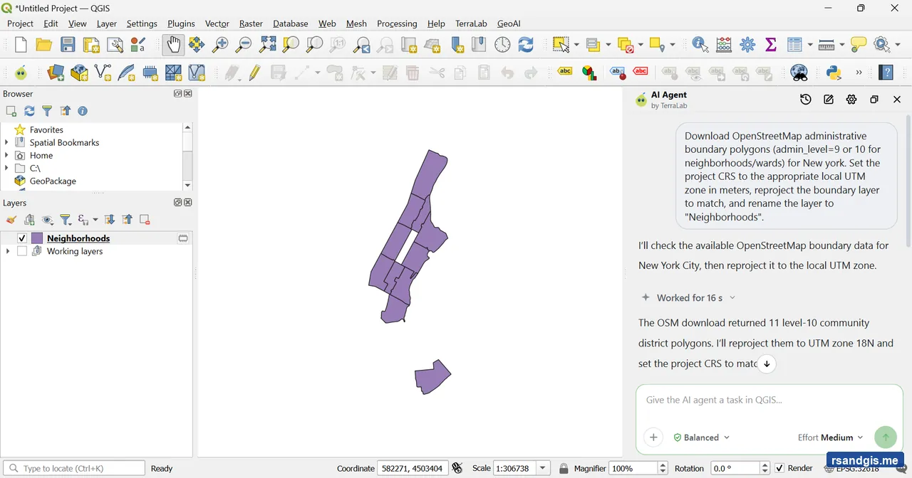
Figure 1: Reprojected OpenStreetMap community district boundaries in UTM Zone 18N (EPSG:32618).
Step 2: Landsat 8/9 LST Retrieval & Conversion
To measure surface temperature variations, thermal infrared remote sensing is essential. We instructed the agent to find a cloud-free summer Landsat scene, isolate the thermal band, clip it, and convert raw digital numbers to degrees Celsius.
"Search the open data catalog for a Landsat 8 or 9 Collection 2 Level-2 scene covering the 'Neighborhoods' layer between 1 June 2026 and 31 August 2026 with less than 10% cloud cover. Load the Surface Temperature band (ST_B10), clip it to 'Neighborhoods', apply the scale factor (multiply by 0.00341802, add 149.0, then subtract 273.15) to convert to degrees Celsius, and name the output raster 'LST_Celsius'."
The agent evaluated available scenes and selected a Landsat 8 acquisition from 23 July 2026 featuring only 2.14% cloud cover. When an initial download hit a local TLS certificate handshake delay, the agent diagnosed the issue and safely completed the download upon user confirmation. It clipped Band 10 (ST_B10) to the Neighborhoods bounding geometry and executed the radiometric conversion formula:
The output raster, named LST_Celsius, retained its native 30-meter spatial resolution, with valid pixel temperatures across the districts ranging from 23.2 °C to 47.8 °C.
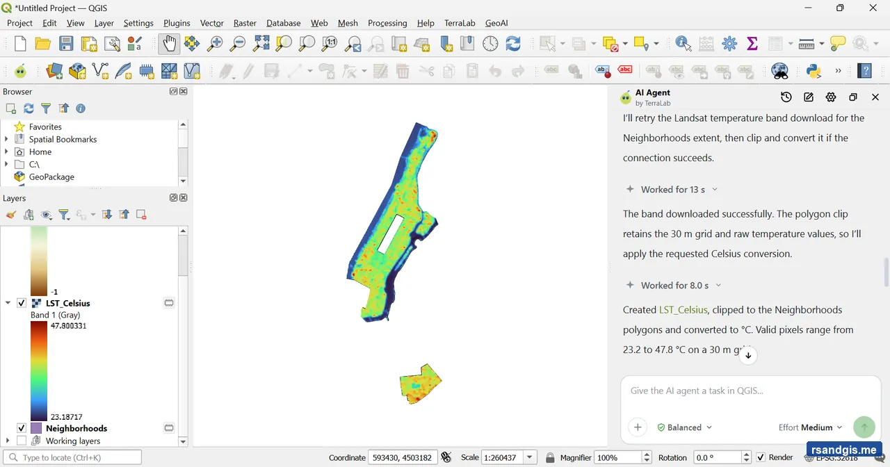
Figure 2: Landsat 8 Land Surface Temperature (LST_Celsius) clipped to community boundaries.
Step 3: Sentinel-2 Multispectral Ingestion & NDVI Calculation
Vegetation canopy provides cooling via shading and evapotranspiration. To quantify green infrastructure, we requested the agent to retrieve Sentinel-2 imagery for the exact same summer window and calculate the Normalized Difference Vegetation Index (NDVI).
"Load Sentinel-2 L2A bands B4 (Red) and B8 (NIR) for the 'Neighborhoods' extent from the same summer period with under 10% cloud cover. Clip both to 'Neighborhoods', calculate the Normalized Difference Vegetation Index using (B8 - B4) / (B8 + B4), and name the resulting layer 'NDVI'."
The agent located a matching Sentinel-2B scene from 23 July 2026 (4.30% cloud cover) that coincided directly with the Landsat pass. It clipped Band 4 (Red, 665 nm) and Band 8 (Near-Infrared, 842 nm) to the neighborhood boundaries on a 10-meter grid and executed the standard index:
The resulting 10-meter raster, NDVI, produced values spanning from -0.80 to 0.99, cleanly delineating asphalt surfaces and water bodies from dense parkland canopies.
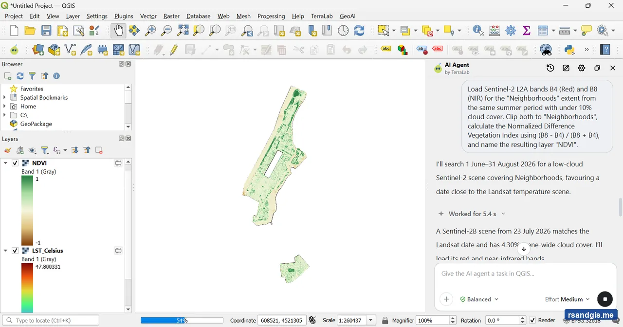
Figure 3: 10m Sentinel-2 NDVI raster highlighting urban tree canopy and parks.
Step 4: Overture Building Density Modeling
High building density increases thermal mass and hinders nocturnal convective cooling. To represent the built environment, the agent was tasked with downloading granular structural footprints and computing building density percentages per district.
"Download building footprints for the 'Neighborhoods' extent using OpenStreetMap or Overture Maps. Calculate the total building footprint area inside each polygon of the 'Neighborhoods' layer, divide it by the polygon's total area to get a building density percentage, and save it as a new attribute field named 'bldg_density'."
TerraLab connected to the Overture Maps Foundation repository, downloading 63,792 individual building footprints across the study area. Crucially, rather than summing individual footprint polygons directly—which could double-count overlapping structures or complex multipart shapes—the agent executed a spatial intersection followed by a geometric union of overlaps before computing area shares. It then added the calculated field bldg_density to the Neighborhoods layer, where density values ranged from 14.11% to 57.46%.
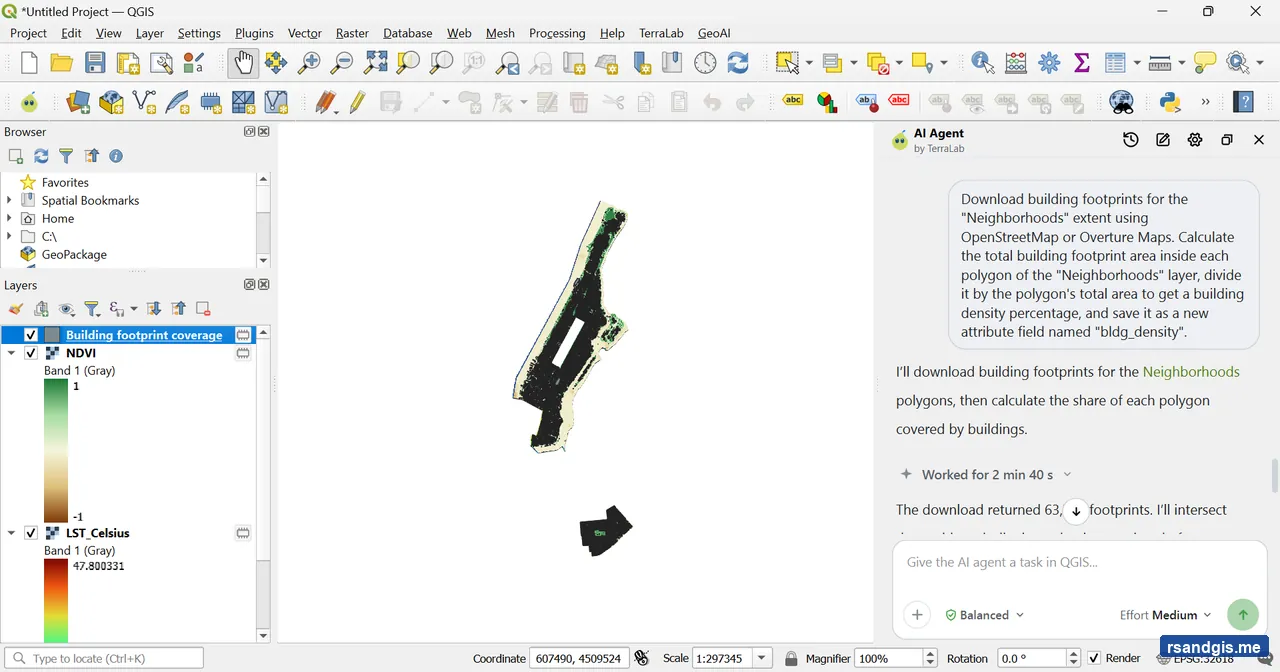
Figure 4: Over 63,000 Overture building footprints unioned to calculate district building density.
Step 5: Zonal Statistics Aggregation
With both satellite rasters and vector building densities prepared, the next phase required summarizing raster values into each district polygon.
"Run Zonal Statistics on the 'Neighborhoods' layer using 'LST_Celsius' to calculate the mean and maximum temperature (prefix 'temp_'), and using 'NDVI' to calculate the mean vegetation index (prefix 'ndvi_')."
The agent executed native QGIS Zonal Statistics in two successive runs, creating three new attributes in the neighborhood attribute table:
temp_mean: Mean surface temperature, ranging from 30.55 °C to 37.85 °C across districts.temp_max: Peak surface temperature per district.ndvi_mean: Mean greenness index, ranging from 0.080 to 0.241.
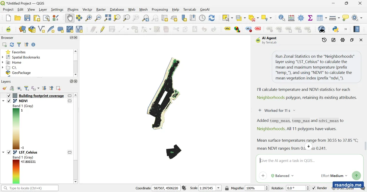
Figure 5: Neighborhood attribute table enriched with zonal temperature and NDVI metrics.
Step 6: Multi-Criteria Evaluation & HVI Scoring
Because raw temperature, NDVI, and building density use entirely different scales, they cannot be combined directly. We instructed the agent to normalize all three variables, invert NDVI so that low vegetation corresponds to high risk, apply weighted coefficients, and isolate the most critical neighborhoods.
"In the 'Neighborhoods' layer, normalize 'temp_mean', 'ndvi_mean', and 'bldg_density' to a 0 to 1 scale using min-max normalization. Invert the normalized NDVI (1 - norm_ndvi) so low vegetation equals high risk. Create a new field named 'HVI_Score' calculated as: (0.5 * norm_temp) + (0.25 * inv_norm_ndvi) + (0.25 * norm_bldg_density). Extract polygons in the top 20% of 'HVI_Score' into a new layer named 'Priority_Vulnerable_Neighborhoods'."
The agent implemented standard min-max scaling across the 11 districts:
It then applied the requested multi-criteria evaluation formula:
Finally, filtering at the 80th percentile isolated the three most acutely vulnerable districts into a dedicated vector layer named Priority_Vulnerable_Neighborhoods:
- Manhattan Community Board 5: HVI Score = 0.771 (highest building density, high surface temperature, minimal canopy).
- Brooklyn Community District 17: HVI Score = 0.628 (elevated temperatures and reduced tree cover).
- Manhattan Community Board 4: HVI Score = 0.544 (intense urban core heating).
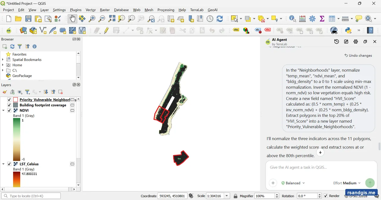
Figure 6: Priority vulnerable neighborhoods isolated at the 80th percentile of HVI_Score.
Step 7: Automated Symbology & Priority Highlighting
To make the analysis interpretable, cartographic styling must emphasize relative risk without obscuring the continuous temperature gradient below.
"Style 'LST_Celsius' with an inverted 'Spectral' ramp at 60% opacity. Style 'Neighborhoods' with a graduated 'YlOrRd' color ramp based on 'HVI_Score' (5 quantiles). Highlight 'Priority_Vulnerable_Neighborhoods' with a thick cyan outline and label them with their name and mean temperature."
The agent applied an inverted Spectral color ramp (blue-green to intense red) to the 30-meter LST raster and adjusted layer transparency to 60%. On the Neighborhoods layer, it set up a 5-class quantile graduated renderer using the Yellow-Orange-Red (YlOrRd) palette. For Priority_Vulnerable_Neighborhoods, it configured a bold 1.2 mm cyan border without fill and attached dynamic data-defined callout labels showing the district name and mean temperature in °C.
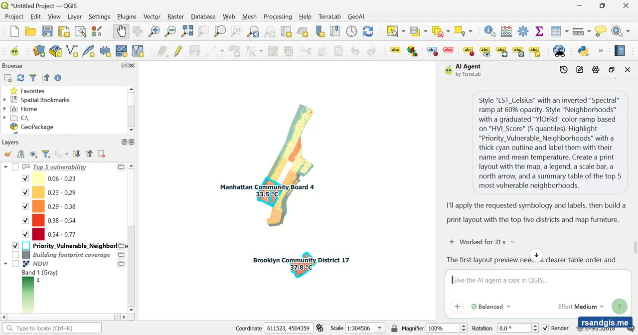
Figure 7: Styled map canvas showing graduated HVI ratings and cyan callouts on priority districts.
Step 8: Cartographic Print Layout Generation
The final step of this tutorial automated the creation of a publication-ready cartographic layout sheet.
"Create a print layout with the map, a legend, a scale bar, a north arrow, and a summary table of the top 5 most vulnerable neighborhoods."
TerraLab constructed an A3 landscape print layout titled Neighborhood heat vulnerability. The layout includes an active map item framed to the district extents, a calibrated metric scale bar, an SVG north arrow, a dynamic legend filtered to active layers, and an automated attribute table listing the top 5 vulnerable neighborhoods alongside their HVI scores and mean surface temperatures.
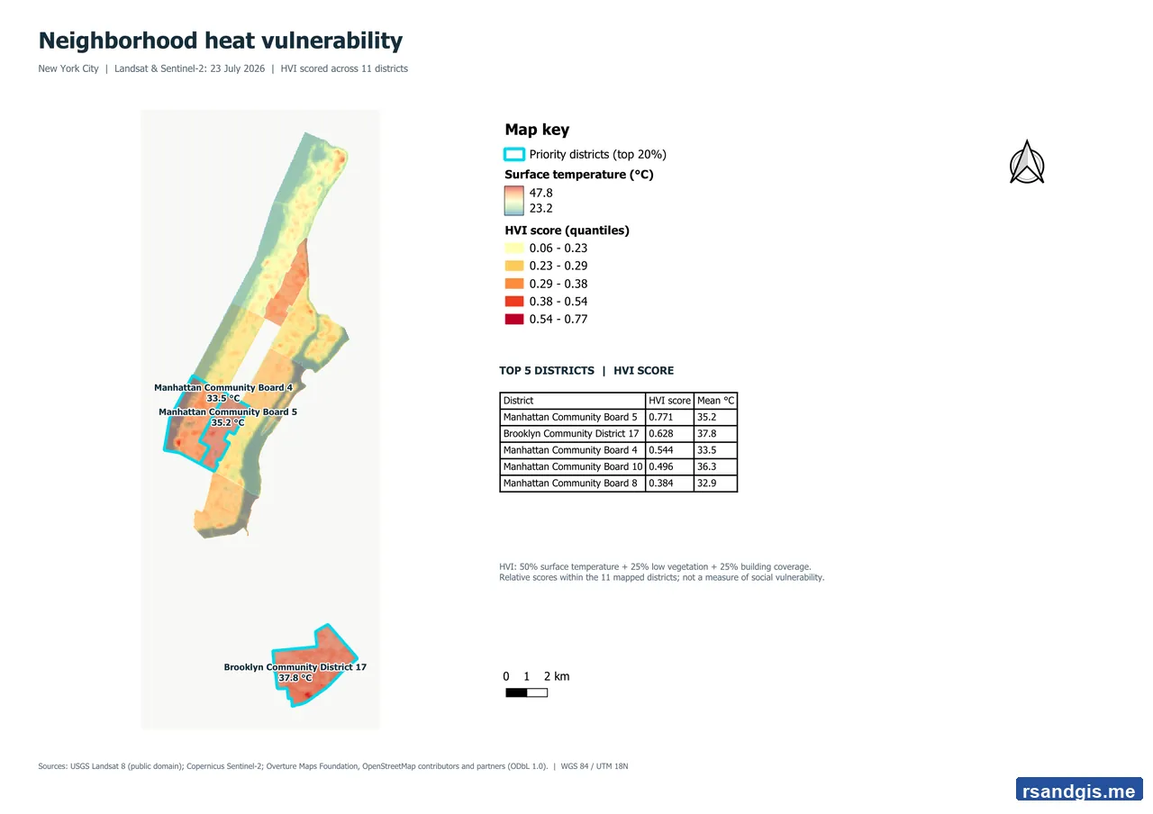
Figure 8: Finished publication-ready print layout map showing vulnerability rankings and spatial furniture.
4. Tutorial 2: Stream Extraction & Watershed Delineation (Soan River)
Hydrological modeling presents a different set of challenges than urban raster overlay. Flat terrain, bridges, digital elevation model (DEM) noise, and artificial sinks can redirect flow paths kilometers away from actual river channels. In this tutorial, the TerraLab AI Agent delineated the entire Soan River Basin (an 11,212.8 km² catchment in the Potohar Plateau of northern Punjab, Pakistan) draining into the Indus River.
Steps 1–2: Copernicus GLO-30 DEM Mosaicking & Planar Reprojection
The agent began by downloading Copernicus WorldDEM GLO-30 elevation data. Because the Soan Basin spans multiple geographic degrees, four tiles were originally mosaicked; after checking the southern boundary, the agent added two additional tiles to ensure complete coverage. The resulting geographic mosaic spanned 6,768 columns by 5,580 rows with zero internal NoData pixels.
Because flow direction routing requires square, metric pixels, the agent executed a GDAL Warp using bilinear resampling to project the mosaic into UTM Zone 43N (EPSG:32643) at a true 30 m × 30 m cell resolution (5,973 × 5,862 grid cells).
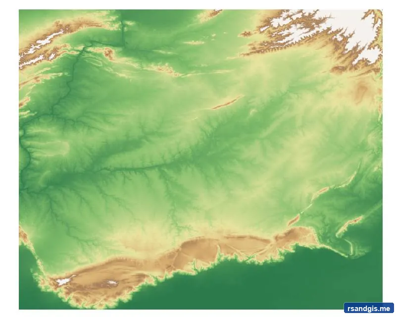
Step 1: Raw 30m DEM mosaic
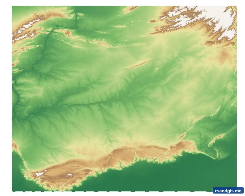
Step 2: Reprojected DEM (EPSG:32643)
Steps 3–5: Depression Evaluation & Initial D8 Routing
In standard hydrology, depression filling is often attempted before routing. The agent tested r.fill.dir and r.terraflow in GRASS GIS. However, r.terraflow generated an unresolved watershed warning, leaving nearly two million zero-direction cells in complex braided terrain. Demonstrating sophisticated reasoning, the agent opted not to force artificial filling, choosing instead to run GRASS r.watershed directly on the projected DEM. Unlike simplistic algorithms, r.watershed utilizes a least-cost search algorithm that routes through depressions internally.
Running with a single-flow-direction (D8) algorithm and a 10,000-cell accumulation threshold, the agent generated initial flow direction and flow accumulation surfaces.
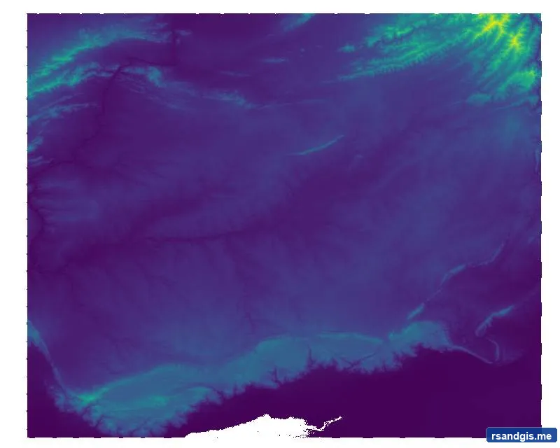
Step 3: Sink filling test
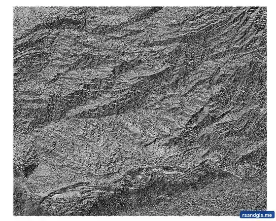
Step 4: Initial D8 flow direction

Step 5: Initial accumulation
Steps 6–7: Confluence Diagnosis & River Hydro-Conditioning
When the agent conducted quality verification on the initial stream routing (Step 6), it discovered a critical real-world discrepancy: the modeled Soan River channel bypassed the mapped OpenStreetMap Indus River confluence by 340 meters, exiting downstream with negative edge-affected accumulation flags.
Rather than proceeding with an incorrect basin outlet, the agent paused, presented the diagnostic mismatch, and proposed hydro-conditioning (stream burning).
Using GRASS r.carve, the agent burned the mapped OpenStreetMap centerlines of the Soan and adjacent Indus into a copy of the DEM. The carving parameters specified a 30-meter stream width and a nominal 5-meter incision depth (lowering 9,991 cells by up to 34.6 meters in steep terrain) to enforce correct channel flow.
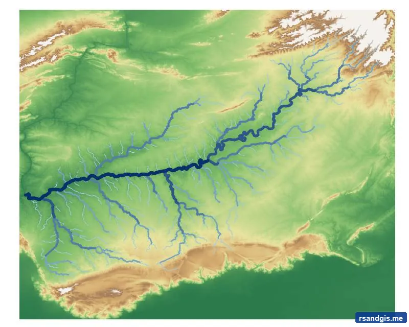
Step 6: Preliminary stream check (340m offset)
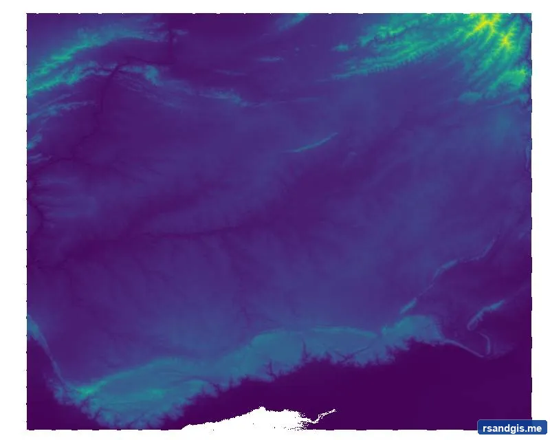
Step 7: River-conditioned DEM (carved)
Steps 8–9: Flow Recalculation on Conditioned Terrain
With the stream network carved into the elevation surface, the agent re-ran GRASS r.watershed. The recalculated flow accumulation surface confirmed that the routed stream channel now aligned within 16.9 meters of the mapped confluence—eliminating the previous 340-meter error and establishing a reliable pour point.
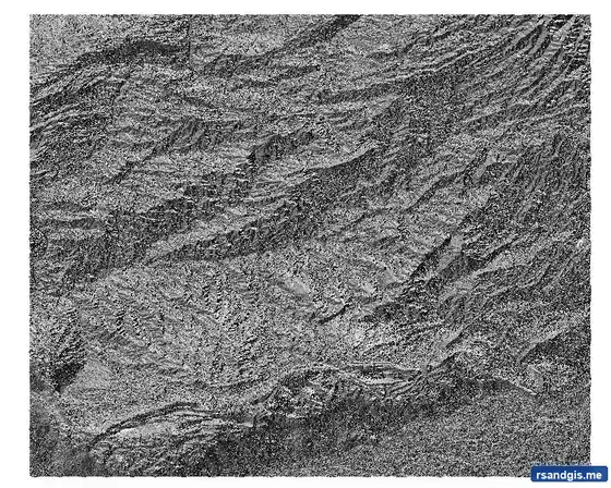
Step 8: Conditioned flow direction
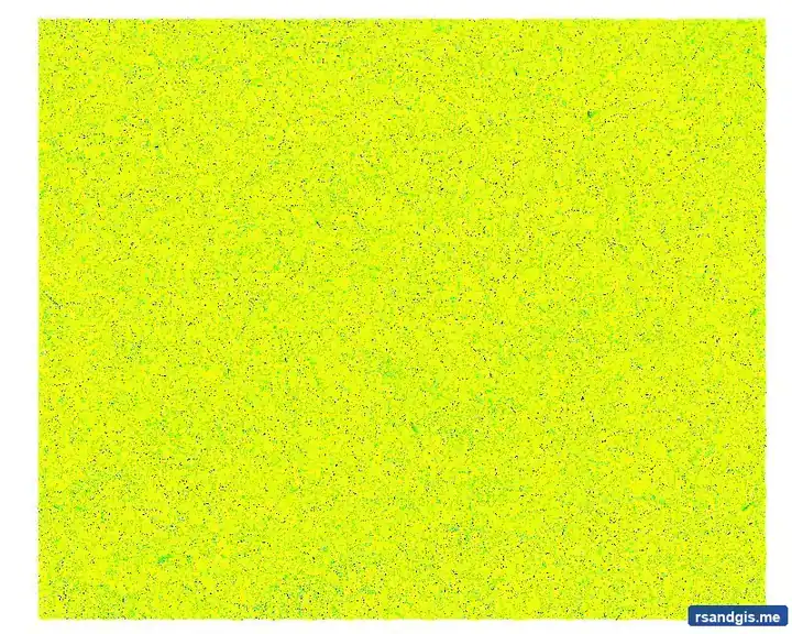
Step 9: Conditioned flow accumulation
Steps 10–12: Pour Point Outlet Masking & Stream Vectorization
With verified flow accumulation, the agent pinpointed the final basin outlet at coordinates 71.720659° E, 33.022494° N and executed GRASS r.water.outlet (Step 10). The resulting catchment mask encompassed 12,464,641 raster cells with zero edge-clipping effects.
In Step 11, the agent polygonized the raster mask using GDAL, repaired geometry slivers, and dissolved the boundaries into a valid multipart basin polygon with an ellipsoidal area of 11,212.8 km².
In Step 12, the accumulation stream network (threshold 10,000 cells) was vectorized using r.to.vect and clipped to the basin boundary, producing 4,235 stream reaches representing the primary tributaries of the Soan River system.
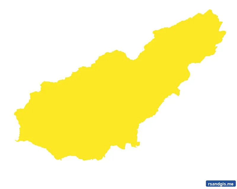
Step 10: Watershed mask
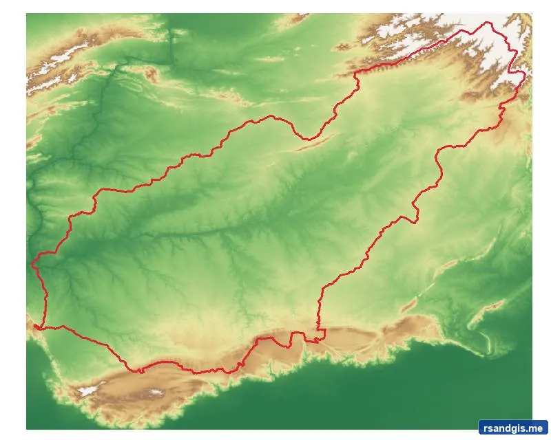
Step 11: Basin boundary
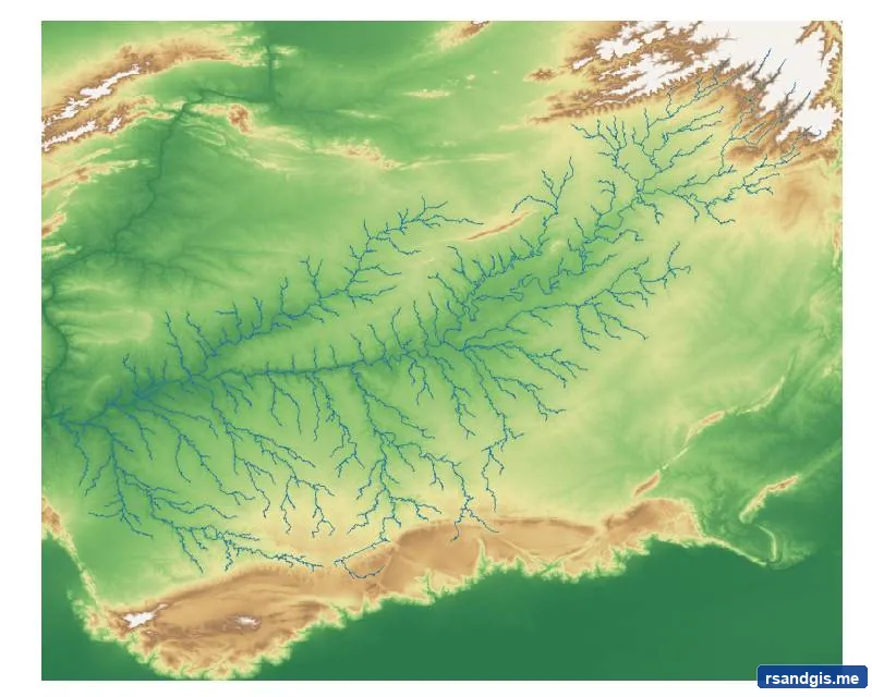
Step 12: Stream network
Step 13: Final Publication Study Area Cartography
To conclude the tutorial, the agent generated a comprehensive A3 study area map. It combined multidirectional hillshade shading, color-ramped elevation, hierarchical blue stream vectors, an explicit catchment outline, geographic coordinate graticules, a north arrow, a scale bar, and complete data citations.
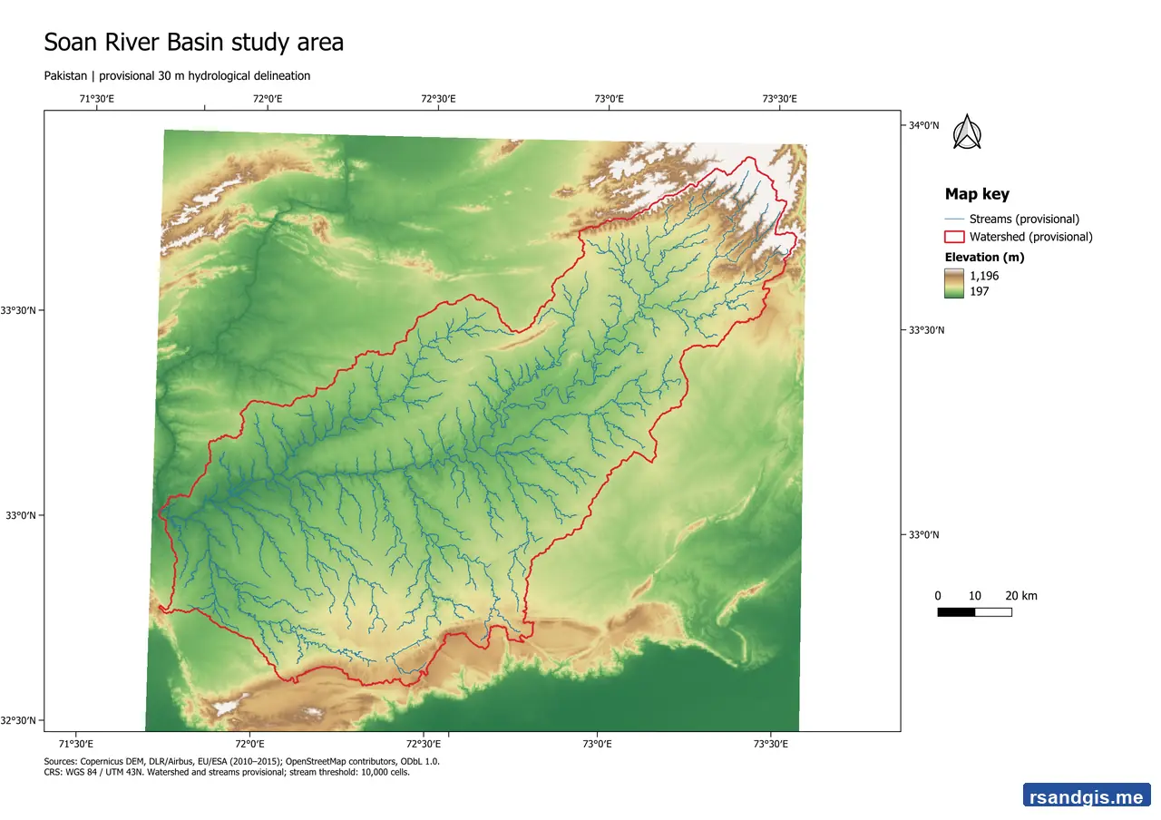
Figure 9: Final cartographic study area map of the Soan River Basin (11,212.8 km²) with stream reaches and hillshade relief.
5. Technical Takeaways & Best Practices
Reviewing both tutorials highlights several crucial insights for professionals looking to incorporate autonomous AI agents into their GIS workflows:
| Workflow Phase | Urban Heat Island (NYC) | Hydrology (Soan Basin) |
|---|---|---|
| Data Domain | Multispectral & Thermal Satellite + Vector Footprints | Digital Elevation Models (DEM) + Stream Centerlines |
| Primary Algorithms | Raster Math, Geometric Union, Zonal Statistics, Min-Max Scaling | GDAL Warp, GRASS r.watershed, r.carve, r.water.outlet |
| Error Handling | TLS certificate retry, date interval confirmation | Sink-fill depression diagnosis, 340m confluence mismatch correction |
| Final Deliverable | Graduated HVI map + A3 vulnerability ranking sheet | 11,212 km² basin boundary + 4,235 stream reaches + A3 map |
Best Practices for Prompting GIS Agents
- Specify Coordinate Reference Systems (CRS) Early: Always instruct the agent to reproject datasets into a local projected metric coordinate system (e.g., UTM) before performing area calculations, buffer queries, or hydrological flow modeling.
- Name Your Output Layers: Explicitly assigning output names (e.g.,
LST_Celsius,Priority_Vulnerable_Neighborhoods) prevents ambiguous layer referencing when executing multi-step pipelines. - Leverage Checkpoints: If an intermediate result shows edge clipping or unexpected styling, use TerraLab's checkpoint restoration rather than manually undoing layers.
- Provide Analytical Boundaries: Providing clear mathematical criteria (e.g., min-max normalization, specific band ratios, or accumulation thresholds) guarantees scientifically sound results.
6. Final Thoughts
To be honest, the TerraLab AI Agent proved to be quite useful across these real-world tests. In the Urban Heat Island & Heat Vulnerability Index workflow, the experience was remarkably smooth: within just 7 to 8 conversational prompts, it completed a comprehensive spatial task that could have taken a significant amount of manual time (though Python execution and importing large datasets can take a few seconds to a couple of minutes).
In regard to the watershed delineation, there was a need for a bit of back-and-forth to apply adjustments and topological fixes. However, from the point of automated data fetching—which is a major plus point for this agent—all the way to cartographic map making and issue resolution, the entire workflow was handled autonomously by the agent.
As a general rule, better prompting and a clearer understanding of context by the AI can minimize errors, which applies directly to this agent as well. For anyone spending hours clicking through nested geoprocessing dialogs, it is an exceptionally useful addition to the modern GIS toolkit. It can act as an autonomous junior analyst working at high speed under your supervision.
7. Frequently Asked Questions (FAQ)
What is the TerraLab AI Agent for QGIS?
The TerraLab AI Agent is an interactive copilot plugin for QGIS. It enables geospatial analysts to execute complete spatial workflows, retrieve open satellite and vector datasets, run GDAL and GRASS algorithms, style layers, and build print layouts using natural language prompts.
How do you install the TerraLab AI Agent in QGIS?
In QGIS, navigate to Plugins > Manage and Install Plugins, search for AI Agent by TerraLab, click Install Plugin, and open the panel using the toolbar icon or the shortcut Ctrl + Alt + A.
What are the core requirements for running TerraLab in QGIS?
You need QGIS 3.28 LTR or later (3.40 LTR recommended) with Python 3, GDAL, and GRASS GIS providers enabled, an active internet connection to download open data from STAC, OSM, and Copernicus, and a free TerraLab account.
Can TerraLab AI Agent handle complex hydrological routing?
Yes. TerraLab orchestrates native GRASS GIS tools like r.watershed, r.carve, and r.water.outlet to perform D8 flow direction, flow accumulation, river burning, and catchment basin delineation.
How does TerraLab handle spatial errors or unverified results?
TerraLab logs every execution step and features checkpoint restoration. When an intermediate output has unresolved edges or network issues, it flags the uncertainty, asks for clarification, and allows you to roll back to any earlier checkpoint.

About the Publisher: Junaid Waseem
Junaid Waseem is a dedicated Remote Sensing and GIS professional holding a Bachelor of Science (BS) in RS & GIS. With a deep passion for geospatial technology, satellite imagery analysis, and spatial data science, Junaid curates high-quality, research-driven content to help professionals and students master the world of Earth observation.